Обсуждение: More stable query plans via more predictable column statistics
Hi Hackers!
This post summarizes a few weeks of research of ANALYZE statistics distribution on one of our bigger production databases with some real-world data and proposes a patch to rectify some of the oddities observed.
Introduction
============
We have observed that for certain data sets the distribution of samples between most_common_vals and histogram_bounds can be unstable: so that it may change dramatically with the next ANALYZE run, thus leading to radically different plans.
I was revisiting the following performance thread and I've found some interesting details about statistics in our environment:
http://www.postgresql.org/message-id/flat/CAMkU=1zxyNMN11YL8G7AGF7k5u4ZHVJN0DqCc_ecO1qs49uJgA@mail.gmail.com#CAMkU=1zxyNMN11YL8G7AGF7k5u4ZHVJN0DqCc_ecO1qs49uJgA@mail.gmail.com
My initial interest was in evaluation if distribution of samples could be made more predictable and less dependent on the factor of luck, thus leading to more stable execution plans.
Unexpected findings
===================
What I have found is that in a significant percentage of instances, when a duplicate sample value is *not* put into the MCV list, it does produce duplicates in the histogram_bounds, so it looks like the MCV cut-off happens too early, even though we have enough space for more values in the MCV list.
In the extreme cases I've found completely empty MCV lists and histograms full of duplicates at the same time, with only about 20% of distinct values in the histogram (as it turns out, this happens due to high fraction of NULLs in the sample).
Data set and approach
=====================
In order to obtain these insights into distribution of statistics samples on one of our bigger databases (~5 TB, 2,300+ tables, 31,000+ individual attributes) I've built some queries which all start with the following CTEs:
WITH stats1 AS (
SELECT *,
current_setting('default_statistics_target')::int stats_target,
array_length(most_common_vals,1) AS num_mcv,
(SELECT SUM(f) FROM UNNEST(most_common_freqs) AS f) AS mcv_frac,
array_length(histogram_bounds,1) AS num_hist,
(SELECT COUNT(DISTINCT h)
FROM UNNEST(histogram_bounds::text::text[]) AS h) AS distinct_hist
FROM pg_stats
WHERE schemaname NOT IN ('pg_catalog', 'information_schema')
),
stats2 AS (
SELECT *,
distinct_hist::float/num_hist AS hist_ratio
FROM stats1
)
The idea here is to collect the number of distinct values in the histogram bounds vs. the total number of bounds. One of the reasons why there might be duplicates in the histogram is a fully occupied MCV list, so we collect the number of MCVs as well, in order to compare it with the stats_target.
These queries assume that all columns use the default statistics target, which was actually the case with the database where I was testing this. (It is straightforward to include per-column stats target in the picture, but to do that efficiently, one will have to copy over the definition of pg_stats view in order to access pg_attribute.attstattarget, and also will have to run this as superuser to access pg_statistic. I wanted to keep the queries simple to make it easier for other interested people to run these queries in their environment, which quite likely excludes superuser access. The more general query is also included[3].)
With the CTEs shown above it was easy to assess the following "meta-statistics":
WITH ...
SELECT count(1),
min(hist_ratio)::real,
avg(hist_ratio)::real,
max(hist_ratio)::real,
stddev(hist_ratio)::real
FROM stats2
WHERE histogram_bounds IS NOT NULL;
-[ RECORD 1 ]----
count | 18980
min | 0.181818
avg | 0.939942
max | 1
stddev | 0.143189
That doesn't look too bad, but the min value is pretty fishy already. If I would run the same query, limiting the scope to non-fully-unique histograms, with "WHERE distinct_hist < num_hist" instead, the picture would be a bit different:
-[ RECORD 1 ]----
count | 3724
min | 0.181818
avg | 0.693903
max | 0.990099
stddev | 0.170845
It shows that about 20% of all analyzed columns that have a histogram (3724/18980), also have some duplicates in it, and that they have only about 70% of distinct sample values on average.
Select statistics examples
==========================
Apart from mere aggregates it is interesting to look at some specific MCVs/histogram examples. The following query is aimed to reconstruct values of certain variables present in analyze.c code of compute_scalar_stats() (again, with the same CTEs as above):
WITH ...
SELECT schemaname ||'.'|| tablename ||'.'|| attname || (CASE inherited WHEN TRUE THEN ' (inherited)' ELSE '' END) AS columnname,
n_distinct, null_frac,
num_mcv, most_common_vals, most_common_freqs,
mcv_frac, (mcv_frac / (1 - null_frac))::real AS nonnull_mcv_frac,
distinct_hist, num_hist, hist_ratio,
histogram_bounds
FROM stats2
ORDER BY hist_ratio
LIMIT 1;
And the worst case as shown by this query (real values replaced with placeholders):
columnname | xxx.yy1.zz1
n_distinct | 22
null_frac | 0.9893
num_mcv |
most_common_vals |
most_common_freqs |
mcv_frac |
nonnull_mcv_frac |
distinct_hist | 4
num_hist | 22
hist_ratio | 0.181818181818182
histogram_bounds | {aaaa,bbb,DDD,DDD,DDD,DDD,DDD,DDD,DDD,DDD,DDD,DDD,DDD,DDD,DDD,DDD,DDD,DDD,DDD,DDD,DDD,zzz}
If one pays attention to the value of null_frac here, it should become apparent that it is the reason of such unexpected picture.
stats_target | num_mcv | mcv_frac | num_hist | hist_ratio
--------------+---------+----------+----------+------------
100 | 100 | 0.849367 | 101 | 0.881188
200 | 200 | 0.964367 | 187 | 0.390374
300 | 294 | 0.998445 | 140 | 1
400 | 307 | 0.998334 | 200 | 1
500 | 329 | 0.998594 | 211 | 1
The MCV list tends to take all available space in this case and hist_ratio hits 100% (after a short drop) and it only requires a small increase in stats_target, compared to the unpatched version. Even if only for this particular distribution pattern, that constitutes an improvement, I believe.
By increasing default_statistics_target on a patched version, I could verify that the number of instances with duplicates in the histogram due to the full MCV lists, which was 1095 at target 100 (see the latest query in prev. section) can be further reduced to down to ~650 at target 500, then ~300 at target 1000. Apparently there always would be distributions which cannot be covered by increasing stats target, but given that histogram fraction also decreases rather dramatically, this should not bother us a lot.
Expected effects on plan stability
==================================
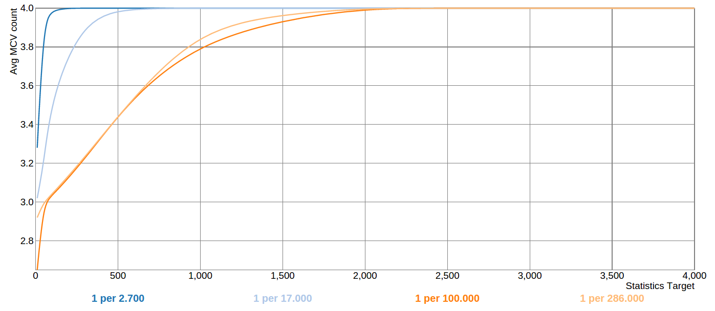
We didn't have a chance to test this change in production, but according to a research by my colleague Stefan Litsche, which is summarized in his blog post[1] (and as it was also presented on PGConf.de last week), with the existing code increasing stats target doesn't always help immediately: in fact for certain distributions it leads to less accurate statistics at first.
If you look at the last graph in that blog, you can see that for very rare values one needs to increase statistics target really high in order to get the rare value covered by statistics reliably. Attached is the same graph, produced from the patched version of the server: now the average number of MCVs for the discussed test distribution shows monotonic increase when increasing statistics target. Also, for this particular case the statistics target can be increased by a much smaller factor in order to get a good sample coverage.
A few word about the patch
==========================
+ /* estimate # of occurrences in sample of a typical value */
+ avgcount = (double) sample_cnt / (double) ndistinct;
Here, ndistinct is the int-type variable, as opposed to the original code where it is re-declared at an inner scope with type double and hides the one from the outer scope. Both sample_cnt and ndistinct decrease with every iteration of the loop, and this average calculation is actually accurate: it's not an estimate.
+
+ /* set minimum threshold count to store a value */
+ mincount = 1.25 * avgcount;
I'm not fond of arbitrary magic coefficients, so I would drop this altogether, but here it goes to make the difference less striking compared to the original code.
I've removed the "mincount < 2" check that was present in the original code, because track[i].count is always >= 2, so it doesn't make a difference if we bump it up to 2 here.
+
+ /* don't let threshold exceed 1/K, however */
+ maxmincount = (sample_cnt - 1) / (double) (num_hist - 1);
Finally, here we cannot set the threshold any higher. As an illustration, consider the following sample (assuming statistics target is > 1):
[A A A A A B B B B B C]
sample_cnt = 11
ndistinct = 3
num_hist = 3
Then maxmincount calculates to (11 - 1) / (3 - 1) = 10 / 2.0 = 5.0.
If we would require the next most common value to be even a tiny bit more popular than this threshold, we would not take the A-sample to the MCV list which we clearly should.
The "take all MCVs" condition
=============================
Finally, the conditions to include all tracked duplicate samples into MCV list look like not all that easy to hit:
- there must be no other non-duplicate values (track_cnt == ndistinct)
- AND there must be no too-wide values, not even a single byte too wide (toowide_cnt == 0)
- AND the estimate of total number of distinct values must not exceed 10% of the total rows in table (stats->stadistinct > 0)
The last condition (track_cnt <= num_mcv) is duplicated from compute_distinct_stats() (former compute_minimal_stats()), but the condition always holds in compute_scalar_stats(), since we never increment track_cnt past num_mcv in this variant of the function.
Each of the above conditions introduces a bifurcation point where one of two very different code paths could be taken. Even though the conditions are strict, with the proposed patch there is no need to relax them if we want to achieve better sample value distribution, because the complex code path has more predictable behavior now.
In conclusion: this code has not been touched for almost 15 years[2] and it might be scary to change anything, but I believe the evidence presented above makes a pretty good argument to attempt improving it.
Thanks for reading, your comments are welcome!
--
Alex
[1] https://tech.zalando.com/blog/analyzing-extreme-distributions-in-postgresql/
[2] http://git.postgresql.org/gitweb/?p=postgresql.git;a=commitdiff;h=b67fc0079cf1f8db03aaa6d16f0ab8bd5d1a240d
b67fc0079cf1f8db03aaa6d16f0ab8bd5d1a240d
Author: Tom Lane <tgl@sss.pgh.pa.us>
Date: Wed Jun 6 21:29:17 2001 +0000
Be a little smarter about deciding how many most-common values to save.
[3] To include per-attribute stattarget, replace the reference to pg_stats view with the following CTE:
WITH stats0 AS (
SELECT s.*,
(CASE a.attstattarget
WHEN -1 THEN current_setting('default_statistics_target')::int
ELSE a.attstattarget END) AS stats_target,
-- from pg_stats view
n.nspname AS schemaname,
c.relname AS tablename,
a.attname,
s.stainherit AS inherited,
s.stanullfrac AS null_frac,
s.stadistinct AS n_distinct,
CASE
WHEN s.stakind1 = 1 THEN s.stavalues1
WHEN s.stakind2 = 1 THEN s.stavalues2
WHEN s.stakind3 = 1 THEN s.stavalues3
WHEN s.stakind4 = 1 THEN s.stavalues4
WHEN s.stakind5 = 1 THEN s.stavalues5
ELSE NULL::anyarray
END AS most_common_vals,
CASE
WHEN s.stakind1 = 1 THEN s.stanumbers1
WHEN s.stakind2 = 1 THEN s.stanumbers2
WHEN s.stakind3 = 1 THEN s.stanumbers3
WHEN s.stakind4 = 1 THEN s.stanumbers4
WHEN s.stakind5 = 1 THEN s.stanumbers5
ELSE NULL::real[]
END AS most_common_freqs,
CASE
WHEN s.stakind1 = 2 THEN s.stavalues1
WHEN s.stakind2 = 2 THEN s.stavalues2
WHEN s.stakind3 = 2 THEN s.stavalues3
WHEN s.stakind4 = 2 THEN s.stavalues4
WHEN s.stakind5 = 2 THEN s.stavalues5
ELSE NULL::anyarray
END AS histogram_bounds
FROM stats_dump_original.pg_statistic AS s
JOIN pg_class c ON c.oid = s.starelid
JOIN pg_attribute a ON c.oid = a.attrelid AND a.attnum = s.staattnum
LEFT JOIN pg_namespace n ON n.oid = c.relnamespace
WHERE NOT a.attisdropped
),
This post summarizes a few weeks of research of ANALYZE statistics distribution on one of our bigger production databases with some real-world data and proposes a patch to rectify some of the oddities observed.
Introduction
============
We have observed that for certain data sets the distribution of samples between most_common_vals and histogram_bounds can be unstable: so that it may change dramatically with the next ANALYZE run, thus leading to radically different plans.
I was revisiting the following performance thread and I've found some interesting details about statistics in our environment:
http://www.postgresql.org/message-id/flat/CAMkU=1zxyNMN11YL8G7AGF7k5u4ZHVJN0DqCc_ecO1qs49uJgA@mail.gmail.com#CAMkU=1zxyNMN11YL8G7AGF7k5u4ZHVJN0DqCc_ecO1qs49uJgA@mail.gmail.com
My initial interest was in evaluation if distribution of samples could be made more predictable and less dependent on the factor of luck, thus leading to more stable execution plans.
Unexpected findings
===================
What I have found is that in a significant percentage of instances, when a duplicate sample value is *not* put into the MCV list, it does produce duplicates in the histogram_bounds, so it looks like the MCV cut-off happens too early, even though we have enough space for more values in the MCV list.
In the extreme cases I've found completely empty MCV lists and histograms full of duplicates at the same time, with only about 20% of distinct values in the histogram (as it turns out, this happens due to high fraction of NULLs in the sample).
Data set and approach
=====================
In order to obtain these insights into distribution of statistics samples on one of our bigger databases (~5 TB, 2,300+ tables, 31,000+ individual attributes) I've built some queries which all start with the following CTEs:
WITH stats1 AS (
SELECT *,
current_setting('default_statistics_target')::int stats_target,
array_length(most_common_vals,1) AS num_mcv,
(SELECT SUM(f) FROM UNNEST(most_common_freqs) AS f) AS mcv_frac,
array_length(histogram_bounds,1) AS num_hist,
(SELECT COUNT(DISTINCT h)
FROM UNNEST(histogram_bounds::text::text[]) AS h) AS distinct_hist
FROM pg_stats
WHERE schemaname NOT IN ('pg_catalog', 'information_schema')
),
stats2 AS (
SELECT *,
distinct_hist::float/num_hist AS hist_ratio
FROM stats1
)
The idea here is to collect the number of distinct values in the histogram bounds vs. the total number of bounds. One of the reasons why there might be duplicates in the histogram is a fully occupied MCV list, so we collect the number of MCVs as well, in order to compare it with the stats_target.
These queries assume that all columns use the default statistics target, which was actually the case with the database where I was testing this. (It is straightforward to include per-column stats target in the picture, but to do that efficiently, one will have to copy over the definition of pg_stats view in order to access pg_attribute.attstattarget, and also will have to run this as superuser to access pg_statistic. I wanted to keep the queries simple to make it easier for other interested people to run these queries in their environment, which quite likely excludes superuser access. The more general query is also included[3].)
With the CTEs shown above it was easy to assess the following "meta-statistics":
WITH ...
SELECT count(1),
min(hist_ratio)::real,
avg(hist_ratio)::real,
max(hist_ratio)::real,
stddev(hist_ratio)::real
FROM stats2
WHERE histogram_bounds IS NOT NULL;
-[ RECORD 1 ]----
count | 18980
min | 0.181818
avg | 0.939942
max | 1
stddev | 0.143189
That doesn't look too bad, but the min value is pretty fishy already. If I would run the same query, limiting the scope to non-fully-unique histograms, with "WHERE distinct_hist < num_hist" instead, the picture would be a bit different:
-[ RECORD 1 ]----
count | 3724
min | 0.181818
avg | 0.693903
max | 0.990099
stddev | 0.170845
It shows that about 20% of all analyzed columns that have a histogram (3724/18980), also have some duplicates in it, and that they have only about 70% of distinct sample values on average.
Select statistics examples
==========================
Apart from mere aggregates it is interesting to look at some specific MCVs/histogram examples. The following query is aimed to reconstruct values of certain variables present in analyze.c code of compute_scalar_stats() (again, with the same CTEs as above):
WITH ...
SELECT schemaname ||'.'|| tablename ||'.'|| attname || (CASE inherited WHEN TRUE THEN ' (inherited)' ELSE '' END) AS columnname,
n_distinct, null_frac,
num_mcv, most_common_vals, most_common_freqs,
mcv_frac, (mcv_frac / (1 - null_frac))::real AS nonnull_mcv_frac,
distinct_hist, num_hist, hist_ratio,
histogram_bounds
FROM stats2
ORDER BY hist_ratio
LIMIT 1;
And the worst case as shown by this query (real values replaced with placeholders):
columnname | xxx.yy1.zz1
n_distinct | 22
null_frac | 0.9893
num_mcv |
most_common_vals |
most_common_freqs |
mcv_frac |
nonnull_mcv_frac |
distinct_hist | 4
num_hist | 22
hist_ratio | 0.181818181818182
histogram_bounds | {aaaa,bbb,DDD,DDD,DDD,DDD,DDD,DDD,DDD,DDD,DDD,DDD,DDD,DDD,DDD,DDD,DDD,DDD,DDD,DDD,DDD,zzz}
If one pays attention to the value of null_frac here, it should become apparent that it is the reason of such unexpected picture.
The code in compute_scalar_stats() goes in such a way that it requires a candidate MCV to count over "samplerows / max(ndistinct / 1.25, num_bins)", but samplerows doesn't account for NULLs, this way we are rejecting would-be MCVs on a wrong basis.
Another, one of the next-to-worst cases (the type of this column is actually TEXT, hence the sort order):
columnname | xxx.yy2.zz2 (inherited)
n_distinct | 30
null_frac | 0
num_mcv | 2
most_common_vals | {101,100}
most_common_freqs | {0.806367,0.1773}
mcv_frac | 0.983667
nonnull_mcv_frac | 0.983667
distinct_hist | 6
num_hist | 28
hist_ratio | 0.214285714285714
histogram_bounds | {202,202,202,202,202,202,202,202,202, *3001*, 302,302,302,302,302,302,302,302,302,302,302, *3031,3185*, 502,502,502,502,502}
(emphasis added around values that are unique)
This time there were no NULLs, but still a lot of duplicates got included in the histogram. This happens because there's relatively small number of distinct values, so the candidate MCVs are limited by "samplerows / num_bins". To really avoid duplicates in the histogram, what we want here is "samplerows / (num_hist - 1)", but this brings a "chicken and egg" problem: we don't know the value of num_hist before we determine the number of MCVs we want to keep.
Solution proposal
=================
The solution I've come up with (and that was also suggested by Jeff Janes in that performance thread mentioned above, as I have now found out) is to move the calculation of the target number of histogram bins inside the loop that evaluates candidate MCVs. At the same time we should account for NULLs more accurately and subtract the MCV counts that we do include in the list, from the count of samples left for the histogram on every loop iteration. A patch implementing this approach is attached.
When I have re-analyzed the worst-case columns with the patch applied, I've got the following picture (some boring stuff in the histogram snipped):
columnname | xxx.yy1.zz1
n_distinct | 21
null_frac | 0.988333
num_mcv | 5
most_common_vals | {DDD,"Rrrrr","Ddddddd","Kkkkkk","Rrrrrrrrrrrrrr"}
most_common_freqs | {0.0108333,0.0001,6.66667e-05,6.66667e-05,6.66667e-05}
mcv_frac | 0.0111333
nonnull_mcv_frac | 0.954287
distinct_hist | 16
num_hist | 16
hist_ratio | 1
histogram_bounds | {aaa,bbb,cccccccc,dddd,"dddd ddddd",Eee,...,zzz}
Now the "DDD" value was treated like an MCV as it should be. This arguably constitutes a bug fix, the rest are probably just improvements.
Here we also see some additional MCVs, which are much less common. Maybe we should also cut them off at some low frequency, but it seems hard to draw a line. I can see that array_typanalyze.c uses a different approach with frequency based cut-off, for example.
The mentioned next-to-worst case becomes:
columnname | xxx.yy2.zz2 (inherited)
n_distinct | 32
null_frac | 0
num_mcv | 15
most_common_vals | {101,100,302,202,502,3001,3059,3029,3031,3140,3041,3095,3100,3102,3192}
most_common_freqs | {0.803933,0.179,0.00656667,0.00526667,0.00356667,0.000333333,0.000133333,0.0001,0.0001,0.0001,6.66667e-05,6.66667e-05,6.66667e-05,6.66667e-05,6.66667e-05}
mcv_frac | 0.999433
nonnull_mcv_frac | 0.999433
distinct_hist | 17
num_hist | 17
hist_ratio | 1
histogram_bounds | {3007,3011,3027,3056,3067,3073,3084,3087,3088,3106,3107,3118,3134,3163,3204,3225,3247}
Now we don't have any duplicates in the histogram at all, and we still have a lot of diversity, i.e. the histogram didn't collapse.
The "meta-statistics" also improves if we re-analyze the whole database with the patch:
(WHERE histogram_bounds IS NOT NULL)
-[ RECORD 1 ]----
count | 18314
min | 0.448276
avg | 0.988884
max | 1
stddev | 0.052899
(WHERE distinct_hist < num_hist)
-[ RECORD 1 ]----
count | 1095
min | 0.448276
avg | 0.81408
max | 0.990099
stddev | 0.119637
We could see that both worst case and average have improved. We did lose some histograms because they have collapsed, but it only constitutes about 3.5% of total count.
We could also see that 100% of instances where we still have duplicates in the histogram are due to the MCV lists being fully occupied:
WITH ...
SELECT count(1), num_mcv = stats_target
FROM stats2
WHERE distinct_hist < num_hist
GROUP BY 2;
-[ RECORD 1 ]--
count | 1095
?column? | t
There's not much left to do but increase statistics target for these columns (or globally).
Increasing stats target
========================
It can be further demonstrated, that with the current code, there are certain data distributions where increasing statistics target doesn't help, in fact for a while it makes things only worse.
I've taken one of the tables where we hit the stats_target limit on the MCV and tried to increase the target gradually, re-analyzing and taking notes of MCV/histogram distribution. The table has around 1.7M rows, but only 950 distinct values in one of the columns.
The results of analyzing the table with different statistics target is as follows:
stats_target | num_mcv | mcv_frac | num_hist | hist_ratio
--------------+---------+----------+----------+------------
100 | 97 | 0.844133 | 101 | 0.841584
200 | 106 | 0.872267 | 201 | 0.771144
300 | 108 | 0.881244 | 301 | 0.528239
400 | 111 | 0.885992 | 376 | 0.422872
500 | 112 | 0.889973 | 411 | 0.396594
1000 | 130 | 0.914046 | 550 | 0.265455
1500 | 167 | 0.938638 | 616 | 0.191558
1625 | 230 | 0.979393 | 570 | 0.161404
1750 | 256 | 0.994913 | 564 | 0.416667
2000 | 260 | 0.996998 | 601 | 0.63228
One can see that num_mcv grows very slowly, while hist_ratio drops significantly and starts growing back only after around stats_target = 1700 in this case. And in order to hit hist_ratio of 100% one would have to analyze the whole table as a "sample", which implies statistics target of around 6000.
If I would do the same test with the patched version, the picture would be dramatically different:
stats_target | num_mcv | mcv_frac | num_hist | hist_ratio
--------------+---------+----------+----------+------------
100 | 100 | 0.849367 | 101 | 0.881188
200 | 200 | 0.964367 | 187 | 0.390374
300 | 294 | 0.998445 | 140 | 1
400 | 307 | 0.998334 | 200 | 1
500 | 329 | 0.998594 | 211 | 1
The MCV list tends to take all available space in this case and hist_ratio hits 100% (after a short drop) and it only requires a small increase in stats_target, compared to the unpatched version. Even if only for this particular distribution pattern, that constitutes an improvement, I believe.
By increasing default_statistics_target on a patched version, I could verify that the number of instances with duplicates in the histogram due to the full MCV lists, which was 1095 at target 100 (see the latest query in prev. section) can be further reduced to down to ~650 at target 500, then ~300 at target 1000. Apparently there always would be distributions which cannot be covered by increasing stats target, but given that histogram fraction also decreases rather dramatically, this should not bother us a lot.
Expected effects on plan stability
==================================
We didn't have a chance to test this change in production, but according to a research by my colleague Stefan Litsche, which is summarized in his blog post[1] (and as it was also presented on PGConf.de last week), with the existing code increasing stats target doesn't always help immediately: in fact for certain distributions it leads to less accurate statistics at first.
If you look at the last graph in that blog, you can see that for very rare values one needs to increase statistics target really high in order to get the rare value covered by statistics reliably. Attached is the same graph, produced from the patched version of the server: now the average number of MCVs for the discussed test distribution shows monotonic increase when increasing statistics target. Also, for this particular case the statistics target can be increased by a much smaller factor in order to get a good sample coverage.
A few word about the patch
==========================
+ /* estimate # of occurrences in sample of a typical value */
+ avgcount = (double) sample_cnt / (double) ndistinct;
Here, ndistinct is the int-type variable, as opposed to the original code where it is re-declared at an inner scope with type double and hides the one from the outer scope. Both sample_cnt and ndistinct decrease with every iteration of the loop, and this average calculation is actually accurate: it's not an estimate.
+
+ /* set minimum threshold count to store a value */
+ mincount = 1.25 * avgcount;
I'm not fond of arbitrary magic coefficients, so I would drop this altogether, but here it goes to make the difference less striking compared to the original code.
I've removed the "mincount < 2" check that was present in the original code, because track[i].count is always >= 2, so it doesn't make a difference if we bump it up to 2 here.
+
+ /* don't let threshold exceed 1/K, however */
+ maxmincount = (sample_cnt - 1) / (double) (num_hist - 1);
Finally, here we cannot set the threshold any higher. As an illustration, consider the following sample (assuming statistics target is > 1):
[A A A A A B B B B B C]
sample_cnt = 11
ndistinct = 3
num_hist = 3
Then maxmincount calculates to (11 - 1) / (3 - 1) = 10 / 2.0 = 5.0.
If we would require the next most common value to be even a tiny bit more popular than this threshold, we would not take the A-sample to the MCV list which we clearly should.
The "take all MCVs" condition
=============================
Finally, the conditions to include all tracked duplicate samples into MCV list look like not all that easy to hit:
- there must be no other non-duplicate values (track_cnt == ndistinct)
- AND there must be no too-wide values, not even a single byte too wide (toowide_cnt == 0)
- AND the estimate of total number of distinct values must not exceed 10% of the total rows in table (stats->stadistinct > 0)
The last condition (track_cnt <= num_mcv) is duplicated from compute_distinct_stats() (former compute_minimal_stats()), but the condition always holds in compute_scalar_stats(), since we never increment track_cnt past num_mcv in this variant of the function.
Each of the above conditions introduces a bifurcation point where one of two very different code paths could be taken. Even though the conditions are strict, with the proposed patch there is no need to relax them if we want to achieve better sample value distribution, because the complex code path has more predictable behavior now.
In conclusion: this code has not been touched for almost 15 years[2] and it might be scary to change anything, but I believe the evidence presented above makes a pretty good argument to attempt improving it.
Thanks for reading, your comments are welcome!
--
Alex
[1] https://tech.zalando.com/blog/analyzing-extreme-distributions-in-postgresql/
[2] http://git.postgresql.org/gitweb/?p=postgresql.git;a=commitdiff;h=b67fc0079cf1f8db03aaa6d16f0ab8bd5d1a240d
b67fc0079cf1f8db03aaa6d16f0ab8bd5d1a240d
Author: Tom Lane <tgl@sss.pgh.pa.us>
Date: Wed Jun 6 21:29:17 2001 +0000
Be a little smarter about deciding how many most-common values to save.
[3] To include per-attribute stattarget, replace the reference to pg_stats view with the following CTE:
WITH stats0 AS (
SELECT s.*,
(CASE a.attstattarget
WHEN -1 THEN current_setting('default_statistics_target')::int
ELSE a.attstattarget END) AS stats_target,
-- from pg_stats view
n.nspname AS schemaname,
c.relname AS tablename,
a.attname,
s.stainherit AS inherited,
s.stanullfrac AS null_frac,
s.stadistinct AS n_distinct,
CASE
WHEN s.stakind1 = 1 THEN s.stavalues1
WHEN s.stakind2 = 1 THEN s.stavalues2
WHEN s.stakind3 = 1 THEN s.stavalues3
WHEN s.stakind4 = 1 THEN s.stavalues4
WHEN s.stakind5 = 1 THEN s.stavalues5
ELSE NULL::anyarray
END AS most_common_vals,
CASE
WHEN s.stakind1 = 1 THEN s.stanumbers1
WHEN s.stakind2 = 1 THEN s.stanumbers2
WHEN s.stakind3 = 1 THEN s.stanumbers3
WHEN s.stakind4 = 1 THEN s.stanumbers4
WHEN s.stakind5 = 1 THEN s.stanumbers5
ELSE NULL::real[]
END AS most_common_freqs,
CASE
WHEN s.stakind1 = 2 THEN s.stavalues1
WHEN s.stakind2 = 2 THEN s.stavalues2
WHEN s.stakind3 = 2 THEN s.stavalues3
WHEN s.stakind4 = 2 THEN s.stavalues4
WHEN s.stakind5 = 2 THEN s.stavalues5
ELSE NULL::anyarray
END AS histogram_bounds
FROM stats_dump_original.pg_statistic AS s
JOIN pg_class c ON c.oid = s.starelid
JOIN pg_attribute a ON c.oid = a.attrelid AND a.attnum = s.staattnum
LEFT JOIN pg_namespace n ON n.oid = c.relnamespace
WHERE NOT a.attisdropped
),
Вложения
"Shulgin, Oleksandr" <oleksandr.shulgin@zalando.de> writes:
> This post summarizes a few weeks of research of ANALYZE statistics
> distribution on one of our bigger production databases with some real-world
> data and proposes a patch to rectify some of the oddities observed.

Please add this to the 2016-01 commitfest ...
        regards, tom lane
On Tue, Dec 1, 2015 at 7:00 PM, Tom Lane <tgl@sss.pgh.pa.us> wrote:
"Shulgin, Oleksandr" <oleksandr.shulgin@zalando.de> writes:
> This post summarizes a few weeks of research of ANALYZE statistics
> distribution on one of our bigger production databases with some real-world
> data and proposes a patch to rectify some of the oddities observed.
Please add this to the 2016-01 commitfest ...
On Tue, Dec 1, 2015 at 10:21 AM, Shulgin, Oleksandr
<oleksandr.shulgin@zalando.de> wrote:
> Hi Hackers!
>
> This post summarizes a few weeks of research of ANALYZE statistics
> distribution on one of our bigger production databases with some real-world
> data and proposes a patch to rectify some of the oddities observed.
>
>
> Introduction
> ============
>
> We have observed that for certain data sets the distribution of samples
> between most_common_vals and histogram_bounds can be unstable: so that it
> may change dramatically with the next ANALYZE run, thus leading to radically
> different plans.
>
> I was revisiting the following performance thread and I've found some
> interesting details about statistics in our environment:
>
>
>
http://www.postgresql.org/message-id/flat/CAMkU=1zxyNMN11YL8G7AGF7k5u4ZHVJN0DqCc_ecO1qs49uJgA@mail.gmail.com#CAMkU=1zxyNMN11YL8G7AGF7k5u4ZHVJN0DqCc_ecO1qs49uJgA@mail.gmail.com
>
> My initial interest was in evaluation if distribution of samples could be
> made more predictable and less dependent on the factor of luck, thus leading
> to more stable execution plans.
>
>
> Unexpected findings
> ===================
>
> What I have found is that in a significant percentage of instances, when a
> duplicate sample value is *not* put into the MCV list, it does produce
> duplicates in the histogram_bounds, so it looks like the MCV cut-off happens
> too early, even though we have enough space for more values in the MCV list.
>
> In the extreme cases I've found completely empty MCV lists and histograms
> full of duplicates at the same time, with only about 20% of distinct values
> in the histogram (as it turns out, this happens due to high fraction of
> NULLs in the sample).

Wow, this is very interesting work.  Using values_cnt rather than
samplerows to compute avgcount seems like a clear improvement.  It
doesn't make any sense to raise the threshold for creating an MCV
based on the presence of additional nulls or too-wide values in the
table.  I bet compute_distinct_stats needs a similar fix.  But for
plan stability considerations, I'd say we should back-patch this all
the way, but those considerations might mitigate for a more restrained
approach.  Still, maybe we should try to sneak at least this much into
9.5 RSN, because I have to think this is going to help people with
mostly-NULL (or mostly-really-wide) columns.

As far as the rest of the fix, your code seems to remove the handling
for ndistinct < 0.  That seems unlikely to be correct, although it's
possible that I am missing something.  Aside from that, the rest of
this seems like a policy change, and I'm not totally sure off-hand
whether it's the right policy.  Having more MCVs can increase planning
time noticeably, and the point of the existing cutoff is to prevent us
from choosing MCVs that aren't actually "C".  I think this change
significantly undermines those protections.  It seems to me that it
might be useful to evaluate the effects of this part of the patch
separately from the samplerows -> values_cnt change.

--
Robert Haas
EnterpriseDB: http://www.enterprisedb.com
The Enterprise PostgreSQL Company
Robert Haas <robertmhaas@gmail.com> writes:
> Still, maybe we should try to sneak at least this much into
> 9.5 RSN, because I have to think this is going to help people with
> mostly-NULL (or mostly-really-wide) columns.

Please no.  We are trying to get to release, not destabilize things.

I think this is fine work for leisurely review and incorporation into
9.6.  It's not appropriate to rush it into 9.5 at the RC stage after
minimal review.
        regards, tom lane
On Fri, Dec 4, 2015 at 6:48 PM, Robert Haas <robertmhaas@gmail.com> wrote:
Wow, this is very interesting work. Using values_cnt rather thanOn Tue, Dec 1, 2015 at 10:21 AM, Shulgin, Oleksandr
<oleksandr.shulgin@zalando.de> wrote:
>
> What I have found is that in a significant percentage of instances, when a
> duplicate sample value is *not* put into the MCV list, it does produce
> duplicates in the histogram_bounds, so it looks like the MCV cut-off happens
> too early, even though we have enough space for more values in the MCV list.
>
> In the extreme cases I've found completely empty MCV lists and histograms
> full of duplicates at the same time, with only about 20% of distinct values
> in the histogram (as it turns out, this happens due to high fraction of
> NULLs in the sample).
samplerows to compute avgcount seems like a clear improvement. It
doesn't make any sense to raise the threshold for creating an MCV
based on the presence of additional nulls or too-wide values in the
table. I bet compute_distinct_stats needs a similar fix.
Yes, and there's also the magic 1.25 multiplier in that code. I think it would make sense to agree first on how exactly the patch for compute_scalar_stats() should look like, then port the relevant bits to compute_distinct_stats().
But for
plan stability considerations, I'd say we should back-patch this all
the way, but those considerations might mitigate for a more restrained
approach. Still, maybe we should try to sneak at least this much into
9.5 RSN, because I have to think this is going to help people with
mostly-NULL (or mostly-really-wide) columns.
I'm not sure. Likely people would complain or have found this out on their own if they were seriously affected.
What I would be interested is people running the queries I've shown on their data to see if there are any interesting/unexpected patterns.
As far as the rest of the fix, your code seems to remove the handling
for ndistinct < 0. That seems unlikely to be correct, although it's
possible that I am missing something.
The difference here is that ndistinct at this scope in the original code did hide a variable from an outer scope. That one could be < 0, but in my code there is no inner-scope ndistinct, we are referring to the outer scope variable which cannot be < 0.
Aside from that, the rest of
this seems like a policy change, and I'm not totally sure off-hand
whether it's the right policy. Having more MCVs can increase planning
time noticeably, and the point of the existing cutoff is to prevent us
from choosing MCVs that aren't actually "C". I think this change
significantly undermines those protections. It seems to me that it
might be useful to evaluate the effects of this part of the patch
separately from the samplerows -> values_cnt change.
Yes, that's why I was wondering if frequency cut-off approach might be helpful here. I'm going to have a deeper look at array's typanalyze implementation at the least.
--
Alex
On Fri, Dec 4, 2015 at 12:53 PM, Tom Lane <tgl@sss.pgh.pa.us> wrote:
> Robert Haas <robertmhaas@gmail.com> writes:
>> Still, maybe we should try to sneak at least this much into
>> 9.5 RSN, because I have to think this is going to help people with
>> mostly-NULL (or mostly-really-wide) columns.
>
> Please no.  We are trying to get to release, not destabilize things.

Well, OK, but I don't really see how that particular bit is anything
other than a bug fix.

--
Robert Haas
EnterpriseDB: http://www.enterprisedb.com
The Enterprise PostgreSQL Company
On Wed, Dec 2, 2015 at 10:20 AM, Shulgin, Oleksandr <oleksandr.shulgin@zalando.de> wrote:
On Tue, Dec 1, 2015 at 7:00 PM, Tom Lane <tgl@sss.pgh.pa.us> wrote:"Shulgin, Oleksandr" <oleksandr.shulgin@zalando.de> writes:
> This post summarizes a few weeks of research of ANALYZE statistics
> distribution on one of our bigger production databases with some real-world
> data and proposes a patch to rectify some of the oddities observed.
Please add this to the 2016-01 commitfest ...
It would be great if some folks could find a moment to run the queries I was showing on their data to confirm (or refute) my findings, or to contribute to the picture in general.
As I was saying, the queries were designed in such a way that even unprivileged user can run them (the results will be limited to the stats data available to that user, obviously; and for custom-tailored statstarget one still needs superuser to join the pg_statistic table directly). Also, on the scale of ~30k attribute statistics records, the queries take only a few seconds to finish.
Cheers!
--
Alex
Tom Lane wrote:
> "Shulgin, Oleksandr" <oleksandr.shulgin@zalando.de> writes:
> > This post summarizes a few weeks of research of ANALYZE statistics
> > distribution on one of our bigger production databases with some real-world
> > data and proposes a patch to rectify some of the oddities observed.
>
> Please add this to the 2016-01 commitfest ...

Tom, are you reviewing this for the current commitfest?

--
Álvaro Herrera                http://www.2ndQuadrant.com/
PostgreSQL Development, 24x7 Support, Remote DBA, Training & Services
Alvaro Herrera <alvherre@2ndquadrant.com> writes:
> Tom Lane wrote:
>> "Shulgin, Oleksandr" <oleksandr.shulgin@zalando.de> writes:
>>> This post summarizes a few weeks of research of ANALYZE statistics
>>> distribution on one of our bigger production databases with some real-world
>>> data and proposes a patch to rectify some of the oddities observed.

>> Please add this to the 2016-01 commitfest ...

> Tom, are you reviewing this for the current commitfest?

Um, I would like to review it, but I doubt I'll find time before the end
of the month.
        regards, tom lane
Hi,

On 01/20/2016 10:49 PM, Alvaro Herrera wrote:
> Tom Lane wrote:
>> "Shulgin, Oleksandr" <oleksandr.shulgin@zalando.de> writes:
>>> This post summarizes a few weeks of research of ANALYZE statistics
>>> distribution on one of our bigger production databases with some real-world
>>> data and proposes a patch to rectify some of the oddities observed.
>>
>> Please add this to the 2016-01 commitfest ...
>
> Tom, are you reviewing this for the current commitfest?

While I'm not the right Tom, I've been looking the the patch recently,
so let me post the review here ...

Firstly, I'd like to appreciate the level of detail of the analysis. I
may disagree with some of the conclusions, but I wish all my patch
submissions were of such high quality.

Regarding the patch itself, I think there's a few different points
raised, so let me discuss them one by one:


1) NULLs vs. MCV threshold
--------------------------

I agree that this seems like a bug, and that we should really compute
the threshold only using non-NULL values. I think the analysis rather
conclusively proves this, and I also think there are places where we do
the same mistake (more on that at the end of the review).


2) mincount = 1.25 * avgcount
-----------------------------

While I share the dislike of arbitrary constants (like the 1.25 here), I
do think we better keep this, otherwise we can just get rid of the
mincount entirely I think - the most frequent value will always be above
the (remaining) average count, making the threshold pointless.

It might have impact in the original code, but in the new one it's quite
useless (see the next point), unless I'm missing some detail.


3) modifying avgcount threshold inside the loop
-----------------------------------------------

The comment was extended with this statement:

  * We also decrease ndistinct in the process such that going forward
  * it refers to the number of distinct values left for the histogram.

and indeed, that's what's happening - at the end of each loop, we do this:

     /* Narrow our view of samples left for the histogram */
     sample_cnt -= track[i].count;
     ndistinct--;

but that immediately lowers the avgcount, as that's re-evaluated within
the same loop

     avgcount = (double) sample_cnt / (double) ndistinct;

which means it's continuously decreasing and lowering the threshold,
although that's partially mitigated by keeping the 1.25 coefficient.

It however makes reasoning about the algorithm much more complicated.


4) for (i = 0; /* i < num_mcv */; i++)
---------------------------------------

The way the loop is coded seems rather awkward, I guess. Not only
there's an unexpected comment in the "for" clause, but the condition
also says this

     /* Another way to say "while (i < num_mcv)" */
     if (i >= num_mcv)
         break;

Why not to write it as a while loop, then? Possibly including the
(num_hist >= 2) condition, like this:

     while ((i < num_mcv) && (num_hist >= 2))
     {
         ...
     }

In any case, the loop would deserve a comment explaining why we think
computing the thresholds like this makes sense.


Summary
-------

Overall, I think this is really about deciding when to cut-off the MCV,
so that it does not grow needlessly large - as Robert pointed out, the
larger the list, the more expensive the estimation (and thus planning).

So even if we could fit the whole sample into the MCV list (i.e. we
believe we've seen all the values and we can fit them into the MCV
list), it may not make sense to do so. The ultimate goal is to estimate
conditions, and if we can do that reasonably even after cutting of the
least frequent values from the MCV list, then why not?

 From this point of view, the analysis concentrates deals just with the
ANALYZE part and does not discuss the estimation counter-part at all.


5) ndistinct estimation vs. NULLs
---------------------------------

While looking at the patch, I started realizing whether we're actually
handling NULLs correctly when estimating ndistinct. Because that part
also uses samplerows directly and entirely ignores NULLs, as it does this:

     numer = (double) samplerows *(double) d;

     denom = (double) (samplerows - f1) +
         (double) f1 *(double) samplerows / totalrows;

     ...
     if (stadistinct > totalrows)
         stadistinct = totalrows;

For tables with large fraction of NULLs, this seems to significantly
underestimate the ndistinct value - for example consider a trivial table
with 95% of NULL values and ~10k distinct values with skewed distribution:

     create table t (id int);

     insert into t
     select (case when random() < 0.05 then (10000 * random() * random())
                  else null end) from generate_series(1,1000000) s(i);

In practice, there are 8325 distinct values in my sample:

     test=# select count(distinct id) from t;
      count
     -------
       8325
     (1 row)

But after ANALYZE with default statistics target (100), ndistinct is
estimated to be ~1300, and with target=1000 the estimate increases to ~6000.

After fixing the estimator to consider fraction of NULLs, the estimates
look like this:

     statistics target |   master  |  patched
    ------------------------------------------
                   100 |     1302  |     5356
                  1000 |     6022  |     6791

So this seems to significantly improve the ndistinct estimate (patch
attached).

regards

--
Tomas Vondra                  http://www.2ndQuadrant.com
PostgreSQL Development, 24x7 Support, Remote DBA, Training & Services
Вложения
On Sat, Jan 23, 2016 at 11:22 AM, Tomas Vondra <tomas.vondra@2ndquadrant.com> wrote:
sample_cnt sample_cnt - track[i].count
------------ > -----------------------------
ndistinct ndistinct - 1
! for (i = 0; i < num_mcv && num_hist >= 2; i++)
Longer MCV lists might be a different story, but see "Increasing stats target" section of the original mail: increasing the target doesn't give quite the expected results with unpatched code either.
Hi,
On 01/20/2016 10:49 PM, Alvaro Herrera wrote:
Tom, are you reviewing this for the current commitfest?
While I'm not the right Tom, I've been looking the the patch recently, so let me post the review here ...
Thank you for the review!
2) mincount = 1.25 * avgcount
-----------------------------
While I share the dislike of arbitrary constants (like the 1.25 here), I do think we better keep this, otherwise we can just get rid of the mincount entirely I think - the most frequent value will always be above the (remaining) average count, making the threshold pointless.
Correct.
It might have impact in the original code, but in the new one it's quite useless (see the next point), unless I'm missing some detail.
3) modifying avgcount threshold inside the loop
-----------------------------------------------
The comment was extended with this statement:
* We also decrease ndistinct in the process such that going forward
* it refers to the number of distinct values left for the histogram.
and indeed, that's what's happening - at the end of each loop, we do this:
/* Narrow our view of samples left for the histogram */
sample_cnt -= track[i].count;
ndistinct--;
but that immediately lowers the avgcount, as that's re-evaluated within the same loop
avgcount = (double) sample_cnt / (double) ndistinct;
which means it's continuously decreasing and lowering the threshold, although that's partially mitigated by keeping the 1.25 coefficient.
I was going to write "not necessarily lowering", but this is actually accurate. The following holds due to track[i].count > avgcount (= sample_cnt / ndistinct):
------------ > -----------------------------
ndistinct ndistinct - 1
It however makes reasoning about the algorithm much more complicated.
Unfortunately, yes.
4) for (i = 0; /* i < num_mcv */; i++)
---------------------------------------
The way the loop is coded seems rather awkward, I guess. Not only there's an unexpected comment in the "for" clause, but the condition also says this
/* Another way to say "while (i < num_mcv)" */
if (i >= num_mcv)
break;
Why not to write it as a while loop, then? Possibly including the (num_hist >= 2) condition, like this:
while ((i < num_mcv) && (num_hist >= 2))
{
...
}
In any case, the loop would deserve a comment explaining why we think computing the thresholds like this makes sense.
This is partially explained by a comment inside the loop:
! for (i = 0; /* i < num_mcv */; i++)
{
! /*
! * We have to put this before the loop condition, otherwise
! * we'll have to repeat this code before the loop and after
! * decreasing ndistinct.
! */
! num_hist = ndistinct;
! if (num_hist > num_bins)
! num_hist = num_bins + 1;
I guess this is a case where code duplication can be traded for more apparent control flow, i.e:
! num_hist = ndistinct;
! if (num_hist > num_bins)
! num_hist = num_bins + 1;
{
...
+ /* Narrow our view of samples left for the histogram */
+ sample_cnt -= track[i].count;
+ ndistinct--;
+
+ num_hist = ndistinct;
+ if (num_hist > num_bins)
+ num_hist = num_bins + 1;
}
Summary
-------
Overall, I think this is really about deciding when to cut-off the MCV, so that it does not grow needlessly large - as Robert pointed out, the larger the list, the more expensive the estimation (and thus planning).
So even if we could fit the whole sample into the MCV list (i.e. we believe we've seen all the values and we can fit them into the MCV list), it may not make sense to do so. The ultimate goal is to estimate conditions, and if we can do that reasonably even after cutting of the least frequent values from the MCV list, then why not?
>From this point of view, the analysis concentrates deals just with the ANALYZE part and does not discuss the estimation counter-part at all.
True, this aspect still needs verification. As stated, my primary motivation was to improve the plan stability for relatively short MCV lists.
5) ndistinct estimation vs. NULLs
---------------------------------
While looking at the patch, I started realizing whether we're actually handling NULLs correctly when estimating ndistinct. Because that part also uses samplerows directly and entirely ignores NULLs, as it does this:
numer = (double) samplerows *(double) d;
denom = (double) (samplerows - f1) +
(double) f1 *(double) samplerows / totalrows;
...
if (stadistinct > totalrows)
stadistinct = totalrows;
For tables with large fraction of NULLs, this seems to significantly underestimate the ndistinct value - for example consider a trivial table with 95% of NULL values and ~10k distinct values with skewed distribution:
create table t (id int);
insert into t
select (case when random() < 0.05 then (10000 * random() * random())
else null end) from generate_series(1,1000000) s(i);
In practice, there are 8325 distinct values in my sample:
test=# select count(distinct id) from t;
count
-------
8325
(1 row)
But after ANALYZE with default statistics target (100), ndistinct is estimated to be ~1300, and with target=1000 the estimate increases to ~6000.
After fixing the estimator to consider fraction of NULLs, the estimates look like this:
statistics target | master | patched
------------------------------------------
100 | 1302 | 5356
1000 | 6022 | 6791
So this seems to significantly improve the ndistinct estimate (patch attached).
Hm... this looks correct. And compute_distinct_stats() needs the same treatment, obviously.
--
Alex
On Mon, Jan 25, 2016 at 5:11 PM, Shulgin, Oleksandr <oleksandr.shulgin@zalando.de> wrote:
>
> On Sat, Jan 23, 2016 at 11:22 AM, Tomas Vondra <tomas.vondra@2ndquadrant.com> wrote:
>>
>>
>> Overall, I think this is really about deciding when to cut-off the MCV, so that it does not grow needlessly large - as Robert pointed out, the larger the list, the more expensive the estimation (and thus planning).
>>
>> So even if we could fit the whole sample into the MCV list (i.e. we believe we've seen all the values and we can fit them into the MCV list), it may not make sense to do so. The ultimate goal is to estimate conditions, and if we can do that reasonably even after cutting of the least frequent values from the MCV list, then why not?
>>
>> From this point of view, the analysis concentrates deals just with the ANALYZE part and does not discuss the estimation counter-part at all.
>
>
> True, this aspect still needs verification. As stated, my primary motivation was to improve the plan stability for relatively short MCV lists.
>
> Longer MCV lists might be a different story, but see "Increasing stats target" section of the original mail: increasing the target doesn't give quite the expected results with unpatched code either.
To address this concern I've run my queries again on the same dataset, now focusing on how the number of MCV items changes with the patched code (using the CTEs from my original mail):
WITH ...
SELECT count(1),
min(num_mcv)::real,
avg(num_mcv)::real,
max(num_mcv)::real,
stddev(num_mcv)::real
FROM stats2
WHERE num_mcv IS NOT NULL;
(ORIGINAL)
count | 27452
min | 1
avg | 32.7115
max | 100
stddev | 40.6927
(PATCHED)
count | 27527
min | 1
avg | 38.4341
max | 100
stddev | 43.3596
A significant portion of the MCV lists is occupying all 100 slots available with the default statistics target, so it also interesting to look at the stats that habe "underfilled" MCV lists (by changing the condition of the WHERE clause to read "num_mcv < 100"):
(<100 ORIGINAL)
count | 20980
min | 1
avg | 11.9541
max | 99
stddev | 18.4132
(<100 PATCHED)
count | 19329
min | 1
avg | 12.3222
max | 99
stddev | 19.6959
As one can see, with the patched code the average length of MCV lists doesn't change all that dramatically, while at the same time exposing all the improvements described in the original mail.
>> After fixing the estimator to consider fraction of NULLs, the estimates look like this:
>>
>> statistics target | master | patched
>> ------------------------------------------
>> 100 | 1302 | 5356
>> 1000 | 6022 | 6791
>>
>> So this seems to significantly improve the ndistinct estimate (patch attached).
>
>
> Hm... this looks correct. And compute_distinct_stats() needs the same treatment, obviously.
I've incorporated this fix into the v2 of my patch, I think it is related closely enough. Also, added corresponding changes to compute_distinct_stats(), which doesn't produce a histogram.
I'm adding this to the next CommitFest. Further reviews are very much appreciated!
--
Alex
>
> On Sat, Jan 23, 2016 at 11:22 AM, Tomas Vondra <tomas.vondra@2ndquadrant.com> wrote:
>>
>>
>> Overall, I think this is really about deciding when to cut-off the MCV, so that it does not grow needlessly large - as Robert pointed out, the larger the list, the more expensive the estimation (and thus planning).
>>
>> So even if we could fit the whole sample into the MCV list (i.e. we believe we've seen all the values and we can fit them into the MCV list), it may not make sense to do so. The ultimate goal is to estimate conditions, and if we can do that reasonably even after cutting of the least frequent values from the MCV list, then why not?
>>
>> From this point of view, the analysis concentrates deals just with the ANALYZE part and does not discuss the estimation counter-part at all.
>
>
> True, this aspect still needs verification. As stated, my primary motivation was to improve the plan stability for relatively short MCV lists.
>
> Longer MCV lists might be a different story, but see "Increasing stats target" section of the original mail: increasing the target doesn't give quite the expected results with unpatched code either.
To address this concern I've run my queries again on the same dataset, now focusing on how the number of MCV items changes with the patched code (using the CTEs from my original mail):
WITH ...
SELECT count(1),
min(num_mcv)::real,
avg(num_mcv)::real,
max(num_mcv)::real,
stddev(num_mcv)::real
FROM stats2
WHERE num_mcv IS NOT NULL;
(ORIGINAL)
count | 27452
min | 1
avg | 32.7115
max | 100
stddev | 40.6927
(PATCHED)
count | 27527
min | 1
avg | 38.4341
max | 100
stddev | 43.3596
A significant portion of the MCV lists is occupying all 100 slots available with the default statistics target, so it also interesting to look at the stats that habe "underfilled" MCV lists (by changing the condition of the WHERE clause to read "num_mcv < 100"):
(<100 ORIGINAL)
count | 20980
min | 1
avg | 11.9541
max | 99
stddev | 18.4132
(<100 PATCHED)
count | 19329
min | 1
avg | 12.3222
max | 99
stddev | 19.6959
As one can see, with the patched code the average length of MCV lists doesn't change all that dramatically, while at the same time exposing all the improvements described in the original mail.
>> After fixing the estimator to consider fraction of NULLs, the estimates look like this:
>>
>> statistics target | master | patched
>> ------------------------------------------
>> 100 | 1302 | 5356
>> 1000 | 6022 | 6791
>>
>> So this seems to significantly improve the ndistinct estimate (patch attached).
>
>
> Hm... this looks correct. And compute_distinct_stats() needs the same treatment, obviously.
I've incorporated this fix into the v2 of my patch, I think it is related closely enough. Also, added corresponding changes to compute_distinct_stats(), which doesn't produce a histogram.
I'm adding this to the next CommitFest. Further reviews are very much appreciated!
--
Alex
Вложения
Hi,

On 02/08/2016 03:01 PM, Shulgin, Oleksandr wrote:>
...
>
> I've incorporated this fix into the v2 of my patch, I think it is
> related closely enough.  Also, added corresponding changes to
> compute_distinct_stats(), which doesn't produce a histogram.

I think it'd be useful not to have all the changes in one lump, but
structure this as a patch series with related changes in separate
chunks. I doubt we'd like to mix the changes in a single commit, and it
makes the reviews and reasoning easier. So those NULL-handling fixes
should be in one patch, the MCV patches in another one.

regards

--
Tomas Vondra                  http://www.2ndQuadrant.com
PostgreSQL Development, 24x7 Support, Remote DBA, Training & Services
On Wed, Feb 24, 2016 at 12:30 AM, Tomas Vondra <tomas.vondra@2ndquadrant.com> wrote:
Hi,
On 02/08/2016 03:01 PM, Shulgin, Oleksandr wrote:
>
...
I've incorporated this fix into the v2 of my patch, I think it is
related closely enough. Also, added corresponding changes to
compute_distinct_stats(), which doesn't produce a histogram.
I think it'd be useful not to have all the changes in one lump, but structure this as a patch series with related changes in separate chunks. I doubt we'd like to mix the changes in a single commit, and it makes the reviews and reasoning easier. So those NULL-handling fixes should be in one patch, the MCV patches in another one.
OK, such a split would make sense to me. Though, I'm a bit late as the commitfest is already closed to new patches, I guess asking the CF manager to split this might work (assuming I produce the patch files)?
--
Alex
On 3/2/16 11:10 AM, Shulgin, Oleksandr wrote:
> On Wed, Feb 24, 2016 at 12:30 AM, Tomas Vondra
> <tomas.vondra@2ndquadrant.com <mailto:tomas.vondra@2ndquadrant.com>> wrote:
>
>     I think it'd be useful not to have all the changes in one lump, but
>     structure this as a patch series with related changes in separate
>     chunks. I doubt we'd like to mix the changes in a single commit, and
>     it makes the reviews and reasoning easier. So those NULL-handling
>     fixes should be in one patch, the MCV patches in another one.
>
>
> OK, such a split would make sense to me.  Though, I'm a bit late as the
> commitfest is already closed to new patches, I guess asking the CF
> manager to split this might work (assuming I produce the patch files)?

If the patch is broken into two files that gives the review/committer
more options but I don't think it requires another CF entry.

--
-David
david@pgmasters.net
On Wed, Mar 2, 2016 at 5:46 PM, David Steele <david@pgmasters.net> wrote:
On 3/2/16 11:10 AM, Shulgin, Oleksandr wrote:
> On Wed, Feb 24, 2016 at 12:30 AM, Tomas Vondra
> <tomas.vondra@2ndquadrant.com <mailto:tomas.vondra@2ndquadrant.com>> wrote:
>
> I think it'd be useful not to have all the changes in one lump, but
> structure this as a patch series with related changes in separate
> chunks. I doubt we'd like to mix the changes in a single commit, and
> it makes the reviews and reasoning easier. So those NULL-handling
> fixes should be in one patch, the MCV patches in another one.
>
>
> OK, such a split would make sense to me. Though, I'm a bit late as the
> commitfest is already closed to new patches, I guess asking the CF
> manager to split this might work (assuming I produce the patch files)?
If the patch is broken into two files that gives the review/committer
more options but I don't think it requires another CF entry.
Alright. I'm attaching the latest version of this patch split in two parts: the first one is NULLs-related bugfix and the second is the "improvement" part, which applies on top of the first one.
--
Alex
Вложения
Shulgin, Oleksandr wrote:

> Alright.  I'm attaching the latest version of this patch split in two
> parts: the first one is NULLs-related bugfix and the second is the
> "improvement" part, which applies on top of the first one.

So is this null-related bugfix supposed to be backpatched?  (I assume
it's not because it's very likely to change existing plans).

--
Álvaro Herrera                http://www.2ndQuadrant.com/
PostgreSQL Development, 24x7 Support, Remote DBA, Training & Services
On Wed, Mar 2, 2016 at 7:33 PM, Alvaro Herrera <alvherre@2ndquadrant.com> wrote:
Shulgin, Oleksandr wrote:
> Alright. I'm attaching the latest version of this patch split in two
> parts: the first one is NULLs-related bugfix and the second is the
> "improvement" part, which applies on top of the first one.
So is this null-related bugfix supposed to be backpatched? (I assume
it's not because it's very likely to change existing plans).
For the good, because cardinality estimations will be more accurate in these cases, so yes I would expect it to be back-patchable.
Alex
On Thu, Mar 3, 2016 at 2:48 AM, Shulgin, Oleksandr
<oleksandr.shulgin@zalando.de> wrote:
> On Wed, Mar 2, 2016 at 7:33 PM, Alvaro Herrera <alvherre@2ndquadrant.com>
> wrote:
>> Shulgin, Oleksandr wrote:
>>
>> > Alright.  I'm attaching the latest version of this patch split in two
>> > parts: the first one is NULLs-related bugfix and the second is the
>> > "improvement" part, which applies on top of the first one.
>>
>> So is this null-related bugfix supposed to be backpatched?  (I assume
>> it's not because it's very likely to change existing plans).
>
> For the good, because cardinality estimations will be more accurate in these
> cases, so yes I would expect it to be back-patchable.

-1.  I think the cost of changing existing query plans in back
branches is too high.  The people who get a better plan never thank
us, but the people who (by bad luck) get a worse plan always complain.

--
Robert Haas
EnterpriseDB: http://www.enterprisedb.com
The Enterprise PostgreSQL Company
On Fri, Mar 4, 2016 at 7:27 PM, Robert Haas <robertmhaas@gmail.com> wrote:
On Thu, Mar 3, 2016 at 2:48 AM, Shulgin, Oleksandr
<oleksandr.shulgin@zalando.de> wrote:
> On Wed, Mar 2, 2016 at 7:33 PM, Alvaro Herrera <alvherre@2ndquadrant.com>
> wrote:
>> Shulgin, Oleksandr wrote:
>>
>> > Alright. I'm attaching the latest version of this patch split in two
>> > parts: the first one is NULLs-related bugfix and the second is the
>> > "improvement" part, which applies on top of the first one.
>>
>> So is this null-related bugfix supposed to be backpatched? (I assume
>> it's not because it's very likely to change existing plans).
>
> For the good, because cardinality estimations will be more accurate in these
> cases, so yes I would expect it to be back-patchable.
-1. I think the cost of changing existing query plans in back
branches is too high. The people who get a better plan never thank
us, but the people who (by bad luck) get a worse plan always complain.
They might get that different plan when they upgrade to the latest major version anyway. Is it set somewhere that minor version upgrades should never affect the planner? I doubt so.
--
Alex
Hi,


On Mon, 2016-03-07 at 12:17 +0100, Shulgin, Oleksandr wrote:
> On Fri, Mar 4, 2016 at 7:27 PM, Robert Haas <robertmhaas@gmail.com>
> wrote:
>         On Thu, Mar 3, 2016 at 2:48 AM, Shulgin, Oleksandr
>         <oleksandr.shulgin@zalando.de> wrote:
>         > On Wed, Mar 2, 2016 at 7:33 PM, Alvaro Herrera
>         <alvherre@2ndquadrant.com>
>         > wrote:
>         >> Shulgin, Oleksandr wrote:
>         >>
>         >> > Alright.  I'm attaching the latest version of this patch
>         split in two
>         >> > parts: the first one is NULLs-related bugfix and the
>         second is the
>         >> > "improvement" part, which applies on top of the first
>         one.
>         >>
>         >> So is this null-related bugfix supposed to be backpatched?
>         (I assume
>         >> it's not because it's very likely to change existing
>         plans).
>         >
>         > For the good, because cardinality estimations will be more
>         accurate in these
>         > cases, so yes I would expect it to be back-patchable.
>
>         -1.  I think the cost of changing existing query plans in back
>         branches is too high.  The people who get a better plan never
>         thank
>         us, but the people who (by bad luck) get a worse plan always
>         complain.
>
>
> They might get that different plan when they upgrade to the latest
> major version anyway.  Is it set somewhere that minor version upgrades
> should never affect the planner?  I doubt so.

Major versions are supposed to add features, which may easily result in
plan changes. Moreover people are expected to do more thorough testing
on major version upgrade, so they're more likely to spot them.

OTOH minor versions are bugfix-only relases, and sometimes the fixes are
security related and people are supposed to install them ASAP. So many
people simply upgrade them without much additional testing and while we
can't promise any of the fixes won't change the plans, we kinda try to
minimize such cases.

That being said, I don't have a clear opinion whether to backpatch this.
I think that it's clearly a bug (especially the first part dealing with
NULL values), and it'd be good to backpatch that. OTOH I can't really
quantify the risks of changing some plans to worse ones.

regards

--
Tomas Vondra                  http://www.2ndQuadrant.com
PostgreSQL Development, 24x7 Support, Remote DBA, Training & Services
On Mon, Mar 7, 2016 at 3:17 AM, Shulgin, Oleksandr
<oleksandr.shulgin@zalando.de> wrote:
> On Fri, Mar 4, 2016 at 7:27 PM, Robert Haas <robertmhaas@gmail.com> wrote:
>>
>> On Thu, Mar 3, 2016 at 2:48 AM, Shulgin, Oleksandr
>> <oleksandr.shulgin@zalando.de> wrote:
>> > On Wed, Mar 2, 2016 at 7:33 PM, Alvaro Herrera
>> > <alvherre@2ndquadrant.com>
>> > wrote:
>> >> Shulgin, Oleksandr wrote:
>> >>
>> >> > Alright.  I'm attaching the latest version of this patch split in two
>> >> > parts: the first one is NULLs-related bugfix and the second is the
>> >> > "improvement" part, which applies on top of the first one.
>> >>
>> >> So is this null-related bugfix supposed to be backpatched?  (I assume
>> >> it's not because it's very likely to change existing plans).
>> >
>> > For the good, because cardinality estimations will be more accurate in
>> > these
>> > cases, so yes I would expect it to be back-patchable.
>>
>> -1.  I think the cost of changing existing query plans in back
>> branches is too high.  The people who get a better plan never thank
>> us, but the people who (by bad luck) get a worse plan always complain.
>
>
> They might get that different plan when they upgrade to the latest major
> version anyway.  Is it set somewhere that minor version upgrades should
> never affect the planner?  I doubt so.

People with meticulous standards are expected to re-validate their
application, including plans and performance, before doing major
version updates into production. They can continue to use a *fully
patched* server from a previous major release while they do that.

This is not the case for minor version updates.  We do not want to put
people in the position where getting a security or corruption-risk
update forces them to also accept changes which may destroy the
performance of their system.

I don't know if it is set out somewhere else, but there are many
examples in this list of us declining to back-patch performance bug
fixes which might negatively impact some users.  The only times we
have done it that I can think of are when there is almost no
conceivable way it could have a meaningful negative effect, or if the
bug was tied in with security or stability bugs that needed to be
fixed anyway and couldn't be separated.

Cheers,

Jeff
On Mon, Mar 7, 2016 at 6:02 PM, Jeff Janes <jeff.janes@gmail.com> wrote:
On Mon, Mar 7, 2016 at 3:17 AM, Shulgin, Oleksandr
<oleksandr.shulgin@zalando.de> wrote:
>
> They might get that different plan when they upgrade to the latest major
> version anyway. Is it set somewhere that minor version upgrades should
> never affect the planner? I doubt so.
People with meticulous standards are expected to re-validate their
application, including plans and performance, before doing major
version updates into production. They can continue to use a *fully
patched* server from a previous major release while they do that.
This is not the case for minor version updates. We do not want to put
people in the position where getting a security or corruption-risk
update forces them to also accept changes which may destroy the
performance of their system.
I don't know if it is set out somewhere else, but there are many
examples in this list of us declining to back-patch performance bug
fixes which might negatively impact some users. The only times we
have done it that I can think of are when there is almost no
conceivable way it could have a meaningful negative effect, or if the
bug was tied in with security or stability bugs that needed to be
fixed anyway and couldn't be separated.
The necessity to perform security upgrades is indeed a valid argument against back-patching this, since this is not a bug that causes incorrect results or data corruption, etc.
Thank you all for the thoughtful replies!
--
Alex
Hi Alex,

Thanks for excellent research.

I've ran your queries against Trustly's production database and I can
confirm your findings, the results are similar:

WITH ...
SELECT count(1),      min(hist_ratio)::real,      avg(hist_ratio)::real,      max(hist_ratio)::real,
stddev(hist_ratio)::realFROM stats2WHERE histogram_bounds IS NOT NULL;

-[ RECORD 1 ]----
count  | 2814
min    | 0.193548
avg    | 0.927357
max    | 1
stddev | 0.164134


WHERE distinct_hist < num_hist
-[ RECORD 1 ]----
count  | 624
min    | 0.193548
avg    | 0.672407
max    | 0.990099
stddev | 0.194901


WITH ..
SELECT schemaname ||'.'|| tablename ||'.'|| attname || (CASE inherited
WHEN TRUE THEN ' (inherited)' ELSE '' END) AS columnname,      n_distinct, null_frac,      num_mcv, most_common_vals,
most_common_freqs,     mcv_frac, (mcv_frac / (1 - null_frac))::real AS nonnull_mcv_frac,      distinct_hist, num_hist,
hist_ratio,     histogram_bounds FROM stats2ORDER BY hist_ratioLIMIT 1;
-[ RECORD 1
]-----+-------------------------------------------------------------------------------------------------------------------------------------------------------------------------------------------------------------------------------------------------------------------------------------------------------------
columnname        | public.x.y
n_distinct        | 103
null_frac         | 0
num_mcv           | 10
most_common_vals  | {0,1,2,3,4,5,6,7,8,9}
most_common_freqs |
{0.4765,0.141733,0.1073,0.0830667,0.0559667,0.0373333,0.0251,0.0188,0.0141,0.0113667}
mcv_frac          | 0.971267
nonnull_mcv_frac  | 0.971267
distinct_hist     | 18
num_hist          | 93
hist_ratio        | 0.193548387096774
histogram_bounds  |

{10,10,10,10,10,10,10,10,10,10,10,10,10,10,10,10,10,10,10,10,10,10,10,10,10,10,10,11,11,11,11,11,11,11,11,11,11,11,11,11,11,11,11,11,11,11,11,12,12,12,12,12,12,12,12,12,12,12,12,13,13,13,13,13,13,13,13,13,13,14,14,14,14,14,15,15,15,15,16,16,16,16,21,23,5074,5437,5830,6049,6496,7046,7784,14629,21285}


On Mon, Jan 18, 2016 at 4:46 PM, Shulgin, Oleksandr
<oleksandr.shulgin@zalando.de> wrote:
> On Wed, Dec 2, 2015 at 10:20 AM, Shulgin, Oleksandr
> <oleksandr.shulgin@zalando.de> wrote:
>>
>> On Tue, Dec 1, 2015 at 7:00 PM, Tom Lane <tgl@sss.pgh.pa.us> wrote:
>>>
>>> "Shulgin, Oleksandr" <oleksandr.shulgin@zalando.de> writes:
>>> > This post summarizes a few weeks of research of ANALYZE statistics
>>> > distribution on one of our bigger production databases with some
>>> > real-world
>>> > data and proposes a patch to rectify some of the oddities observed.
>>>
>>> Please add this to the 2016-01 commitfest ...
>>
>>
>> Added: https://commitfest.postgresql.org/8/434/
>
>
> It would be great if some folks could find a moment to run the queries I was
> showing on their data to confirm (or refute) my findings, or to contribute
> to the picture in general.
>
> As I was saying, the queries were designed in such a way that even
> unprivileged user can run them (the results will be limited to the stats
> data available to that user, obviously; and for custom-tailored statstarget
> one still needs superuser to join the pg_statistic table directly).  Also,
> on the scale of ~30k attribute statistics records, the queries take only a
> few seconds to finish.
>
> Cheers!
> --
> Alex
>


--
Joel Jacobson

Mobile: +46703603801
Trustly.com | Newsroom | LinkedIn | Twitter
On Tue, Mar 8, 2016 at 3:36 PM, Joel Jacobson <joel@trustly.com> wrote:
Hi Alex,
Thanks for excellent research.
Joel,
Thank you for spending your time to run these :-)
I've ran your queries against Trustly's production database and I can
confirm your findings, the results are similar:
WITH ...
SELECT count(1),
min(hist_ratio)::real,
avg(hist_ratio)::real,
max(hist_ratio)::real,
stddev(hist_ratio)::real
FROM stats2
WHERE histogram_bounds IS NOT NULL;
-[ RECORD 1 ]----
count | 2814
min | 0.193548
avg | 0.927357
max | 1
stddev | 0.164134
WHERE distinct_hist < num_hist
-[ RECORD 1 ]----
count | 624
min | 0.193548
avg | 0.672407
max | 0.990099
stddev | 0.194901
WITH ..
SELECT schemaname ||'.'|| tablename ||'.'|| attname || (CASE inherited
WHEN TRUE THEN ' (inherited)' ELSE '' END) AS columnname,
n_distinct, null_frac,
num_mcv, most_common_vals, most_common_freqs,
mcv_frac, (mcv_frac / (1 - null_frac))::real AS nonnull_mcv_frac,
distinct_hist, num_hist, hist_ratio,
histogram_bounds
FROM stats2
ORDER BY hist_ratio
LIMIT 1;
-[ RECORD 1 ]-----+-------------------------------------------------------------------------------------------------------------------------------------------------------------------------------------------------------------------------------------------------------------------------------------------------------------
columnname | public.x.y
n_distinct | 103
null_frac | 0
num_mcv | 10
most_common_vals | {0,1,2,3,4,5,6,7,8,9}
most_common_freqs |
{0.4765,0.141733,0.1073,0.0830667,0.0559667,0.0373333,0.0251,0.0188,0.0141,0.0113667}
mcv_frac | 0.971267
nonnull_mcv_frac | 0.971267
distinct_hist | 18
num_hist | 93
hist_ratio | 0.193548387096774
histogram_bounds |
{10,10,10,10,10,10,10,10,10,10,10,10,10,10,10,10,10,10,10,10,10,10,10,10,10,10,10,11,11,11,11,11,11,11,11,11,11,11,11,11,11,11,11,11,11,11,11,12,12,12,12,12,12,12,12,12,12,12,12,13,13,13,13,13,13,13,13,13,13,14,14,14,14,14,15,15,15,15,16,16,16,16,21,23,5074,5437,5830,6049,6496,7046,7784,14629,21285}
I don't want to be asking for too much here, but is there a chance you could try the effects of the proposed patch on an offline copy of your database?
Do you envision or maybe have experienced problems with query plans referring to the columns that are near the top of the above hist_ratio report? In other words: what are the practical implications for you with the values being duplicated rather badly throughout the histogram like in the example you shown?
Thank you!
--
Alex
On Wed, Jan 20, 2016 at 5:09 PM, Tom Lane <tgl@sss.pgh.pa.us> wrote:
> Alvaro Herrera <alvherre@2ndquadrant.com> writes:
>> Tom Lane wrote:
>>> "Shulgin, Oleksandr" <oleksandr.shulgin@zalando.de> writes:
>>>> This post summarizes a few weeks of research of ANALYZE statistics
>>>> distribution on one of our bigger production databases with some real-world
>>>> data and proposes a patch to rectify some of the oddities observed.
>
>>> Please add this to the 2016-01 commitfest ...
>
>> Tom, are you reviewing this for the current commitfest?
>
> Um, I would like to review it, but I doubt I'll find time before the end
> of the month.

Tom, can you pick this up?

--
Robert Haas
EnterpriseDB: http://www.enterprisedb.com
The Enterprise PostgreSQL Company
On Wed, Mar 9, 2016 at 1:25 AM, Shulgin, Oleksandr
<oleksandr.shulgin@zalando.de> wrote:
> Thank you for spending your time to run these :-)

n/p, it took like 30 seconds :-)

> I don't want to be asking for too much here, but is there a chance you could
> try the effects of the proposed patch on an offline copy of your database?

Yes, I think that should be possible.

> Do you envision or maybe have experienced problems with query plans
> referring to the columns that are near the top of the above hist_ratio
> report?  In other words: what are the practical implications for you with
> the values being duplicated rather badly throughout the histogram like in
> the example you shown?

I don't know much about the internals of query planner,
I just read the "57.1. Row Estimation Examples" to get a basic understanding.

If I understand it correctly, if the histogram_bounds contains a lot
of duplicated values,
then the row estimation will be inaccurate, which in turn will trick
the query planner
into a sub-optimal plan?

We've had some problems lately with the query planner, or actually we've always
had them but never noticed them nor cared about them, but now during peak times
we've had short periods where we haven't been able to fully cope up
with the traffic.

I tracked down the most self_time-consuming functions and quickly saw
how to optimize them.
Many of them where on the form:
SELECT .. FROM SomeBigTable WHERE Col1 = [some dynamic value] AND Col2
= [some constant value] AND Col3 = [some other constant value]
The number of rows matching the WHERE clause were very tiny, perfect
match for a partial index:
CREATE INDEX .. ON SomeBigTable USING btree (Col1) WHERE Col2 = [some
constant value] AND Col3 = [some other constant value];

Even though the new partial index matched the query perfectly, the
query planner didn't want to use it. Instead it continued to use some
other sub-optimal index.

The only way to force it to use the correct index was to use the
"+0"-trick which I recently learned from one of my colleagues:
SELECT .. FROM SomeBigTable WHERE Col1 = [some dynamic value] AND
Col2+0 = [some constant value] AND Col3+0 = [some other constant
value]
CREATE INDEX .. ON SomeBigTable USING btree (Col1) WHERE Col2+0 =
[some constant value] AND Col3+0 = [some other constant value];

By adding +0 to the columns, the query planner will as I understand it
be extremely motivated to use the correct index, as otherwise it would
have to do a seq scan on the entire big table, which would be very
costly.

I'm glad the trick worked, now the system is fast again.

We're still on 9.1, so maybe these problems will go away once we upgrade to 9.5.

I don't know if these problems I described can be fixed by your patch,
but I wanted to share this story since I know our systems (Trustly's
and Zalando's) are quite similar in design,
so maybe you have experienced something similar.

(Side note: My biggest wish would be some way to specify explicitly on
a per top-level function level a list of indexes the query planner is
allowed to consider or is NOT allowed to consider.)
Shulgin, Oleksandr wrote:

> Alright.  I'm attaching the latest version of this patch split in two
> parts: the first one is NULLs-related bugfix and the second is the
> "improvement" part, which applies on top of the first one.

I went over patch 0001 and it seems pretty reasonable.  It's missing
some comment updates -- at least the large comments that talk about Duj1
should be modified to indicate why the code is now subtracting the null
count.  Also, I can't quite figure out why the "else" now in line 2131
is now "else if track_cnt != 0".  What happens if track_cnt is zero?
The comment above the "if" block doesn't provide any guidance.

--
Álvaro Herrera                http://www.2ndQuadrant.com/
PostgreSQL Development, 24x7 Support, Remote DBA, Training & Services
Robert Haas <robertmhaas@gmail.com> writes:
> On Wed, Jan 20, 2016 at 5:09 PM, Tom Lane <tgl@sss.pgh.pa.us> wrote:
>> Um, I would like to review it, but I doubt I'll find time before the end
>> of the month.

> Tom, can you pick this up?

Yes, now that I've gotten out from under the pathification thing,
I have cycles for patch review.  I'll take this one.
        regards, tom lane
On Tue, Mar 8, 2016 at 9:10 PM, Joel Jacobson <joel@trustly.com> wrote:
On Wed, Mar 9, 2016 at 1:25 AM, Shulgin, Oleksandr
<oleksandr.shulgin@zalando.de> wrote:
> Thank you for spending your time to run these :-)
n/p, it took like 30 seconds :-)
Great! I'm glad to hear it was as easy to use as I hoped for :-)
> I don't want to be asking for too much here, but is there a chance you could
> try the effects of the proposed patch on an offline copy of your database?
Yes, I think that should be possible.
> Do you envision or maybe have experienced problems with query plans
> referring to the columns that are near the top of the above hist_ratio
> report? In other words: what are the practical implications for you with
> the values being duplicated rather badly throughout the histogram like in
> the example you shown?
I don't know much about the internals of query planner,
I just read the "57.1. Row Estimation Examples" to get a basic understanding.
If I understand it correctly, if the histogram_bounds contains a lot
of duplicated values,
then the row estimation will be inaccurate, which in turn will trick
the query planner
into a sub-optimal plan?
Yes, basically it should matter the most for the equality comparison operator, such that a MCV entry would provide more accurate selectivity estimate (and the histogram is not used at all in this case anyway). For the "less/greater-than" comparison both MCV list and histogram are used, so the drawback of having repeated values in the histogram, in my understanding is the same: less accurate selectivity estimates for the values that could fall precisely into a bin which didn't make it into the histogram.
We've had some problems lately with the query planner, or actually we've always
had them but never noticed them nor cared about them, but now during peak times
we've had short periods where we haven't been able to fully cope up
with the traffic.
I tracked down the most self_time-consuming functions and quickly saw
how to optimize them.
Many of them where on the form:
SELECT .. FROM SomeBigTable WHERE Col1 = [some dynamic value] AND Col2
= [some constant value] AND Col3 = [some other constant value]
The number of rows matching the WHERE clause were very tiny, perfect
match for a partial index:
CREATE INDEX .. ON SomeBigTable USING btree (Col1) WHERE Col2 = [some
constant value] AND Col3 = [some other constant value];
Even though the new partial index matched the query perfectly, the
query planner didn't want to use it. Instead it continued to use some
other sub-optimal index.
The only way to force it to use the correct index was to use the
"+0"-trick which I recently learned from one of my colleagues:
SELECT .. FROM SomeBigTable WHERE Col1 = [some dynamic value] AND
Col2+0 = [some constant value] AND Col3+0 = [some other constant
value]
CREATE INDEX .. ON SomeBigTable USING btree (Col1) WHERE Col2+0 =
[some constant value] AND Col3+0 = [some other constant value];
By adding +0 to the columns, the query planner will as I understand it
be extremely motivated to use the correct index, as otherwise it would
have to do a seq scan on the entire big table, which would be very
costly.
I'm glad the trick worked, now the system is fast again.
We're still on 9.1, so maybe these problems will go away once we upgrade to 9.5.
Hm... sounds like a planner bug to me. I'm not exceptionally aware of the changes in partial index handling that were made after 9.1, though grepping the commit log for "partial index" produces a number of hits after the date of 9.1 release.
I don't know if these problems I described can be fixed by your patch,
but I wanted to share this story since I know our systems (Trustly's
and Zalando's) are quite similar in design,
so maybe you have experienced something similar.
I would not expect this type of problem to be affected by the patch in any way, though maybe I'm missing the complete picture here.
Also, I'm not aware of similar problems in our systems, but I can ask around. :-)
Thank you.
--
Alex
On Tue, Mar 8, 2016 at 8:16 PM, Alvaro Herrera <alvherre@2ndquadrant.com> wrote:
Shulgin, Oleksandr wrote:
> Alright. I'm attaching the latest version of this patch split in two
> parts: the first one is NULLs-related bugfix and the second is the
> "improvement" part, which applies on top of the first one.
I went over patch 0001 and it seems pretty reasonable. It's missing
some comment updates -- at least the large comments that talk about Duj1
should be modified to indicate why the code is now subtracting the null
count.
Good point.
Also, I can't quite figure out why the "else" now in line 2131
is now "else if track_cnt != 0". What happens if track_cnt is zero?
The comment above the "if" block doesn't provide any guidance.
It is there only to avoid potentially dividing zero by zero when calculating avgcount (which will not be used after that anyway). I agree it deserves a comment.
Thank you!
--
Alex
Hi,

On Wed, 2016-03-09 at 10:58 +0100, Shulgin, Oleksandr wrote:
> On Tue, Mar 8, 2016 at 9:10 PM, Joel Jacobson <joel@trustly.com>
> wrote:
>         On Wed, Mar 9, 2016 at 1:25 AM, Shulgin, Oleksandr
>         <oleksandr.shulgin@zalando.de> wrote:
>         > Thank you for spending your time to run these :-)
>
>         n/p, it took like 30 seconds :-)
>
>
> Great!  I'm glad to hear it was as easy to use as I hoped for :-)
>
>
>         > I don't want to be asking for too much here, but is there a
>         chance you could
>         > try the effects of the proposed patch on an offline copy of
>         your database?
>
>         Yes, I think that should be possible.
>
>         > Do you envision or maybe have experienced problems with
>         query plans
>         > referring to the columns that are near the top of the above
>         hist_ratio
>         > report?  In other words: what are the practical implications
>         for you with
>         > the values being duplicated rather badly throughout the
>         histogram like in
>         > the example you shown?
>
>         I don't know much about the internals of query planner,
>         I just read the "57.1. Row Estimation Examples" to get a basic
>         understanding.
>
>         If I understand it correctly, if the histogram_bounds contains
>         a lot
>         of duplicated values,
>         then the row estimation will be inaccurate, which in turn will
>         trick
>         the query planner
>         into a sub-optimal plan?
>
>
> Yes, basically it should matter the most for the equality comparison
> operator, such that a MCV entry would provide more accurate
> selectivity estimate (and the histogram is not used at all in this
> case anyway).  For the "less/greater-than" comparison both MCV list
> and histogram are used, so the drawback of having repeated values in
> the histogram, in my understanding is the same: less accurate
> selectivity estimates for the values that could fall precisely into a
> bin which didn't make it into the histogram.
>
>
>         We've had some problems lately with the query planner, or
>         actually we've always
>         had them but never noticed them nor cared about them, but now
>         during peak times
>         we've had short periods where we haven't been able to fully
>         cope up
>         with the traffic.
>
>         I tracked down the most self_time-consuming functions and
>         quickly saw
>         how to optimize them.
>         Many of them where on the form:
>         SELECT .. FROM SomeBigTable WHERE Col1 = [some dynamic value]
>         AND Col2
>         = [some constant value] AND Col3 = [some other constant value]
>         The number of rows matching the WHERE clause were very tiny,
>         perfect
>         match for a partial index:
>         CREATE INDEX .. ON SomeBigTable USING btree (Col1) WHERE Col2
>         = [some
>         constant value] AND Col3 = [some other constant value];
>
>         Even though the new partial index matched the query perfectly,
>         the
>         query planner didn't want to use it. Instead it continued to
>         use some
>         other sub-optimal index.
>
>         The only way to force it to use the correct index was to use
>         the
>         "+0"-trick which I recently learned from one of my colleagues:
>         SELECT .. FROM SomeBigTable WHERE Col1 = [some dynamic value]
>         AND
>         Col2+0 = [some constant value] AND Col3+0 = [some other
>         constant
>         value]
>         CREATE INDEX .. ON SomeBigTable USING btree (Col1) WHERE Col2
>         +0 =
>         [some constant value] AND Col3+0 = [some other constant
>         value];
>
>         By adding +0 to the columns, the query planner will as I
>         understand it
>         be extremely motivated to use the correct index, as otherwise
>         it would
>         have to do a seq scan on the entire big table, which would be
>         very
>         costly.
>
>         I'm glad the trick worked, now the system is fast again.
>
>         We're still on 9.1, so maybe these problems will go away once
>         we upgrade to 9.5.
>
>
> Hm... sounds like a planner bug to me.  I'm not exceptionally aware of
> the changes in partial index handling that were made after 9.1, though
> grepping the commit log for "partial index" produces a number of hits
> after the date of 9.1 release.

My first guess would be this is related to the costing bug addressed in
   https://commitfest.postgresql.org/9/299/

I.e. the planner is not accounting for the index predicate correctly,
and ends up choosing the full index. It'd be interesting to see if the
patch makes the optimizer to choose the right index in your example.

The fact that +0 fixes the issue however seems a bit contradictory,
though. That forces the planner to use default selectivity estimates
(~5% for equality expressions, IIRC), not the per-column statistics.

Combined with the independence assumption for multiple AND clauses, this
may easily confuse the planner. I'd expect that would affect both
indexes equally, but perhaps not.

Would be useful to see explain analyze - it's not clear what you mean by
"the number of rows matching WHERE were tiny", whether an estimate or
the actual number.

regards

--
Tomas Vondra                  http://www.2ndQuadrant.com
PostgreSQL Development, 24x7 Support, Remote DBA, Training & Services
Hi,

On Wed, 2016-03-09 at 11:23 +0100, Shulgin, Oleksandr wrote:
> On Tue, Mar 8, 2016 at 8:16 PM, Alvaro Herrera
> <alvherre@2ndquadrant.com> wrote:
>         Shulgin, Oleksandr wrote:
>
>         > Alright.  I'm attaching the latest version of this patch
>         split in two
>         > parts: the first one is NULLs-related bugfix and the second
>         is the
>         > "improvement" part, which applies on top of the first one.
>
>         I went over patch 0001 and it seems pretty reasonable.  It's
>         missing
>         some comment updates -- at least the large comments that talk
>         about Duj1
>         should be modified to indicate why the code is now subtracting
>         the null
>         count.
>
>
> Good point.
>
>
>         Also, I can't quite figure out why the "else" now in line 2131
>         is now "else if track_cnt != 0".  What happens if track_cnt is
>         zero?
>         The comment above the "if" block doesn't provide any guidance.
>
>
> It is there only to avoid potentially dividing zero by zero when
> calculating avgcount (which will not be used after that anyway).  I
> agree it deserves a comment.

That definitely deserves a comment. It's not immediately clear why
(track_cnt != 0) would prevent division by zero in the code. The only
way such error could happen is if ndistinct==0, because that's the
actual denominator. Which means this
   ndistinct = ndistinct * sample_cnt

would have to evaluate to 0. But ndistinct==0 can't happen as we're in
the (nonnull_cnt > 0) branch, and that guarantees (standistinct != 0).

Thus the only possibility seems to be (nonnull_cnt==toowide_cnt). Why
not to use this condition instead?

FWIW while looking at the code I noticed that we skip wide varlena
values but not cstrings. Seems a bit suspicious.

regards

--
Tomas Vondra                  http://www.2ndQuadrant.com
PostgreSQL Development, 24x7 Support, Remote DBA, Training & Services
Tomas Vondra wrote:

> FWIW while looking at the code I noticed that we skip wide varlena
> values but not cstrings. Seems a bit suspicious.

Uh, can you actually have columns of cstring type?  I don't think you
can ...

--
Álvaro Herrera                http://www.2ndQuadrant.com/
PostgreSQL Development, 24x7 Support, Remote DBA, Training & Services
On Wed, 2016-03-09 at 12:02 -0300, Alvaro Herrera wrote:
> Tomas Vondra wrote:
>
> > FWIW while looking at the code I noticed that we skip wide varlena
> > values but not cstrings. Seems a bit suspicious.
>
> Uh, can you actually have columns of cstring type?  I don't think you
> can ...

Yeah, but then why do we handle that in compute_scalar_stats?

--
Tomas Vondra                  http://www.2ndQuadrant.com
PostgreSQL Development, 24x7 Support, Remote DBA, Training & Services
Tomas Vondra <tomas.vondra@2ndquadrant.com> writes:
> On Wed, 2016-03-09 at 12:02 -0300, Alvaro Herrera wrote:
>> Tomas Vondra wrote:
>>> FWIW while looking at the code I noticed that we skip wide varlena
>>> values but not cstrings. Seems a bit suspicious.

>> Uh, can you actually have columns of cstring type?  I don't think you
>> can ...

> Yeah, but then why do we handle that in compute_scalar_stats?

If you're looking at what I think you're looking at, we aren't bothering
because we assume that cstrings won't be very wide.  Since they're not
toastable or compressable, they certainly won't exceed BLCKSZ.
        regards, tom lane
On Wed, Mar 9, 2016 at 1:33 PM, Tomas Vondra <tomas.vondra@2ndquadrant.com> wrote:
Hi,
On Wed, 2016-03-09 at 11:23 +0100, Shulgin, Oleksandr wrote:
> On Tue, Mar 8, 2016 at 8:16 PM, Alvaro Herrera
> <alvherre@2ndquadrant.com> wrote:
>
> Also, I can't quite figure out why the "else" now in line 2131
> is now "else if track_cnt != 0". What happens if track_cnt is
> zero?
> The comment above the "if" block doesn't provide any guidance.
>
>
> It is there only to avoid potentially dividing zero by zero when
> calculating avgcount (which will not be used after that anyway). I
> agree it deserves a comment.
That definitely deserves a comment. It's not immediately clear why
(track_cnt != 0) would prevent division by zero in the code. The only
way such error could happen is if ndistinct==0, because that's the
actual denominator. Which means this
ndistinct = ndistinct * sample_cnt
would have to evaluate to 0. But ndistinct==0 can't happen as we're in
the (nonnull_cnt > 0) branch, and that guarantees (standistinct != 0).
Thus the only possibility seems to be (nonnull_cnt==toowide_cnt). Why
not to use this condition instead?
Yes, I now recall that my actual concern was that sample_cnt may calculate to 0 due to the latest condition above, but that also implies track_cnt == 0, and then we have a for loop there which will not run at all due to this, so I figured we can avoid calculating avgcount and running the loop altogether with that check. I'm not opposed to changing the condition if that makes the code easier to understand (or dropping it altogether if calculating 0/0 is believed to be harmless anyway).
--
Alex
"Shulgin, Oleksandr" <oleksandr.shulgin@zalando.de> writes:
> Yes, I now recall that my actual concern was that sample_cnt may calculate
> to 0 due to the latest condition above, but that also implies track_cnt ==
> 0, and then we have a for loop there which will not run at all due to this,
> so I figured we can avoid calculating avgcount and running the loop
> altogether with that check.  I'm not opposed to changing the condition if
> that makes the code easier to understand (or dropping it altogether if
> calculating 0/0 is believed to be harmless anyway).

Avoiding intentional zero divides is good.  It might happen to work
conveniently on your machine, but I wouldn't think it's portable.
        regards, tom lane
On Wed, Mar 9, 2016 at 5:28 PM, Tom Lane <tgl@sss.pgh.pa.us> wrote:
"Shulgin, Oleksandr" <oleksandr.shulgin@zalando.de> writes:
> Yes, I now recall that my actual concern was that sample_cnt may calculate
> to 0 due to the latest condition above, but that also implies track_cnt ==
> 0, and then we have a for loop there which will not run at all due to this,
> so I figured we can avoid calculating avgcount and running the loop
> altogether with that check. I'm not opposed to changing the condition if
> that makes the code easier to understand (or dropping it altogether if
> calculating 0/0 is believed to be harmless anyway).
Avoiding intentional zero divides is good. It might happen to work
conveniently on your machine, but I wouldn't think it's portable.
Tom,
Thank you for volunteering to review this patch!
Are you waiting on me to produce an updated version with more comments about NULL-handling in the distinct estimator, or do you have something cooking already?
--
Regards,
Alex
On Tue, Mar 15, 2016 at 4:47 PM, Shulgin, Oleksandr <oleksandr.shulgin@zalando.de> wrote:
On Wed, Mar 9, 2016 at 5:28 PM, Tom Lane <tgl@sss.pgh.pa.us> wrote:"Shulgin, Oleksandr" <oleksandr.shulgin@zalando.de> writes:
> Yes, I now recall that my actual concern was that sample_cnt may calculate
> to 0 due to the latest condition above, but that also implies track_cnt ==
> 0, and then we have a for loop there which will not run at all due to this,
> so I figured we can avoid calculating avgcount and running the loop
> altogether with that check. I'm not opposed to changing the condition if
> that makes the code easier to understand (or dropping it altogether if
> calculating 0/0 is believed to be harmless anyway).
Avoiding intentional zero divides is good. It might happen to work
conveniently on your machine, but I wouldn't think it's portable.Tom,Thank you for volunteering to review this patch!Are you waiting on me to produce an updated version with more comments about NULL-handling in the distinct estimator, or do you have something cooking already?
I've just seen that this patch doesn't have a reviewer assigned anymore...
I would welcome any review. If we don't commit even the first part (bugfix) now, is it going to be 9.7-only material?..
--
Alex
"Shulgin, Oleksandr" <oleksandr.shulgin@zalando.de> writes:
> I've just seen that this patch doesn't have a reviewer assigned anymore...

I took my name off it because I was busy with other things and didn't
want to discourage other people from reviewing it meanwhile.  I do hope
to get to it eventually but there's a lot of stuff on my to-do list.

> I would welcome any review.

Me too.
        regards, tom lane
On Tue, Mar 29, 2016 at 6:24 PM, Tom Lane <tgl@sss.pgh.pa.us> wrote:
"Shulgin, Oleksandr" <oleksandr.shulgin@zalando.de> writes:
> I've just seen that this patch doesn't have a reviewer assigned anymore...
I took my name off it because I was busy with other things and didn't
want to discourage other people from reviewing it meanwhile.
I wanted to write that this should not be stopping anyone else from attempting a review, but then learned that you have removed your name. ;-)
I do hope
to get to it eventually but there's a lot of stuff on my to-do list.
Completely understood.
Thank you.
--
Alex
"Shulgin, Oleksandr" <oleksandr.shulgin@zalando.de> writes:
> Alright.  I'm attaching the latest version of this patch split in two
> parts: the first one is NULLs-related bugfix and the second is the
> "improvement" part, which applies on top of the first one.

I've applied the first of these patches, broken into two parts first
because it seemed like there were two issues and second because Tomas
deserved primary credit for one part, ie realizing we were using the
Haas-Stokes formula wrong.

As for the other part, I committed it with one non-cosmetic change:
I do not think it is right to omit "too wide" values when considering
the threshold for MCVs.  As submitted, the patch was inconsistent on
that point anyway since it did it differently in compute_distinct_stats
and compute_scalar_stats.  But the larger picture here is that we define
the MCV population to exclude nulls, so it's reasonable to consider a
value as an MCV even if it's greatly outnumbered by nulls.  There is
no such exclusion for "too wide" values; those things are just an
implementation limitation in analyze.c, not something that is part of
the pg_statistic definition.  If there are a lot of "too wide" values
in the sample, we don't know whether any of them are duplicates, but
we do know that the frequencies of the normal-width values have to be
discounted appropriately.

Haven't looked at 0002 yet.
        regards, tom lane
<p dir="ltr">On Apr 1, 2016 23:14, "Tom Lane" <<a href="mailto:tgl@sss.pgh.pa.us">tgl@sss.pgh.pa.us</a>>
wrote:<br/> ><br /> > "Shulgin, Oleksandr" <<a
href="mailto:oleksandr.shulgin@zalando.de">oleksandr.shulgin@zalando.de</a>>writes:<br /> > > Alright.  I'm
attachingthe latest version of this patch split in two<br /> > > parts: the first one is NULLs-related bugfix and
thesecond is the<br /> > > "improvement" part, which applies on top of the first one.<br /> ><br /> > I've
appliedthe first of these patches,<p dir="ltr">Great news, thank you!<p dir="ltr">> broken into two parts first<br
/>> because it seemed like there were two issues and second because Tomas<br /> > deserved primary credit for one
part,ie realizing we were using the<br /> > Haas-Stokes formula wrong.<br /> ><br /> > As for the other part,
Icommitted it with one non-cosmetic change:<br /> > I do not think it is right to omit "too wide" values when
considering<br/> > the threshold for MCVs.  As submitted, the patch was inconsistent on<br /> > that point anyway
sinceit did it differently in compute_distinct_stats<br /> > and compute_scalar_stats.  But the larger picture here
isthat we define<br /> > the MCV population to exclude nulls, so it's reasonable to consider a<br /> > value as
anMCV even if it's greatly outnumbered by nulls.  There is<br /> > no such exclusion for "too wide" values; those
thingsare just an<br /> > implementation limitation in analyze.c, not something that is part of<br /> > the
pg_statisticdefinition.  If there are a lot of "too wide" values<br /> > in the sample, we don't know whether any of
themare duplicates, but<br /> > we do know that the frequencies of the normal-width values have to be<br /> >
discountedappropriately.<p dir="ltr">Okay.<p dir="ltr">> Haven't looked at 0002 yet.<p dir="ltr">[crosses fingers]
hopeyou'll have a chance to do that before feature freeze for 9.6…<p dir="ltr">--<br /> Alex<br />
"Shulgin, Oleksandr" <oleksandr.shulgin@zalando.de> writes:
> On Apr 1, 2016 23:14, "Tom Lane" <tgl@sss.pgh.pa.us> wrote:
>> Haven't looked at 0002 yet.

> [crosses fingers] hope you'll have a chance to do that before feature
> freeze for 9.6

I studied this patch for awhile after rebasing it onto yesterday's
commits.  I did not like the fact that the compute_scalar_stats logic
would allow absolutely anything into the MCV list once num_hist falls
below 2.  I think it's important that we continue to reject values that
are only seen once in the sample, because there's no very good reason to
think that they are MCVs and not just infrequent values that by luck
appeared in the sample.  However, after I rearranged the tests there so
that "if (num_hist >= 2)" only controlled whether to apply the 1/K limit,
one of the regression tests started to fail: there's a place in
rowsecurity.sql that expects that if a column contains nothing but several
instances of a single value, that value will be recorded as a lone MCV.
Now this isn't a particularly essential thing for that test, but it still
seems like a good property for ANALYZE to have.  The reason it's failing,
of course, is that the test as written cannot possibly accept the last
(or only) value.

Before I noticed the regression failure, I'd been thinking that maybe it'd
be better if the decision rule were not "at least 100+x% of the average
frequency of this value and later ones", but "at least 100+x% of the
average frequency of values after this one".  With that formulation, we're
not constrained as to the range of x.  Now, if there are *no* values after
this one, then this way needs an explicit special case in order not to
compute 0/0; but the preceding para shows that we need a special case for
the last value anyway.

So, attached is a patch rewritten along these lines.  I used 50% rather
than 25% as the new cutoff percentage --- obviously it should be higher
in this formulation than before, but I have no idea if that particular
number is good or we should use something else.  Also, the rule for the
last value is "at least 1% of the non-null samples".  That's a pure guess
as well.

I do not have any good corpuses of data to try this on.  Can folks who
have been following this thread try it on their data and see how it
does?  Also please try some other multipliers besides 1.5, so we can
get a feeling for where that cutoff should be placed.

            regards, tom lane

diff --git a/src/backend/commands/analyze.c b/src/backend/commands/analyze.c
index 44a4b3f..a2c606b 100644
*** a/src/backend/commands/analyze.c
--- b/src/backend/commands/analyze.c
*************** compute_distinct_stats(VacAttrStatsP sta
*** 2120,2128 ****
           * we are able to generate a complete MCV list (all the values in the
           * sample will fit, and we think these are all the ones in the table),
           * then do so.  Otherwise, store only those values that are
!          * significantly more common than the (estimated) average. We set the
!          * threshold rather arbitrarily at 25% more than average, with at
!          * least 2 instances in the sample.
           */
          if (track_cnt < track_max && toowide_cnt == 0 &&
              stats->stadistinct > 0 &&
--- 2120,2138 ----
           * we are able to generate a complete MCV list (all the values in the
           * sample will fit, and we think these are all the ones in the table),
           * then do so.  Otherwise, store only those values that are
!          * significantly more common than the ones we omit.  We determine that
!          * by considering the values in frequency order, and accepting each
!          * one if it is at least 50% more common than the average among the
!          * values after it.  The 50% threshold is somewhat arbitrary.
!          *
!          * Note that the 50% rule will never accept a value with count 1,
!          * since all the values have count at least 1; this is a property we
!          * desire, since there's no very good reason to assume that a
!          * single-occurrence value is an MCV and not just a random non-MCV.
!          *
!          * We need a special rule for the very last value.  If we get to it,
!          * we'll accept it if it's at least 1% of the non-null samples and has
!          * count more than 1.
           */
          if (track_cnt < track_max && toowide_cnt == 0 &&
              stats->stadistinct > 0 &&
*************** compute_distinct_stats(VacAttrStatsP sta
*** 2133,2153 ****
          }
          else
          {
!             /* d here is the same as d in the Haas-Stokes formula */
              int            d = nonnull_cnt - summultiple + nmultiple;
!             double        avgcount,
!                         mincount;

!             /* estimate # occurrences in sample of a typical nonnull value */
!             avgcount = (double) nonnull_cnt / (double) d;
!             /* set minimum threshold count to store a value */
!             mincount = avgcount * 1.25;
!             if (mincount < 2)
!                 mincount = 2;
              if (num_mcv > track_cnt)
                  num_mcv = track_cnt;
              for (i = 0; i < num_mcv; i++)
              {
                  if (track[i].count < mincount)
                  {
                      num_mcv = i;
--- 2143,2181 ----
          }
          else
          {
!             /* d here is initially the same as d in the Haas-Stokes formula */
              int            d = nonnull_cnt - summultiple + nmultiple;
!             int            remaining_samples = nonnull_cnt;

!             /* can't store more MCVs than we tracked ... */
              if (num_mcv > track_cnt)
                  num_mcv = track_cnt;
+             /* locate first value we're not going to store as an MCV */
              for (i = 0; i < num_mcv; i++)
              {
+                 double        avgcount,
+                             mincount;
+
+                 /* remove current value from remaining_samples and d */
+                 remaining_samples -= track[i].count;
+                 d--;
+                 if (d > 0)
+                 {
+                     /* get avg # occurrences of distinct values after this */
+                     avgcount = (double) remaining_samples / (double) d;
+                     /* set minimum count to accept a value (is surely > 1) */
+                     mincount = avgcount * 1.50;
+                 }
+                 else
+                 {
+                     /* last value, use 1% rule */
+                     mincount = nonnull_cnt * 0.01;
+
+                     /* here, we need a clamp to avoid accepting count 1 */
+                     if (mincount < 2)
+                         mincount = 2;
+                 }
+                 /* if this value falls below threshold, we're done */
                  if (track[i].count < mincount)
                  {
                      num_mcv = i;
*************** compute_scalar_stats(VacAttrStatsP stats
*** 2375,2381 ****
                          /*
                           * Found a new item for the mcv list; find its
                           * position, bubbling down old items if needed. Loop
!                          * invariant is that j points at an empty/ replaceable
                           * slot.
                           */
                          int            j;
--- 2403,2409 ----
                          /*
                           * Found a new item for the mcv list; find its
                           * position, bubbling down old items if needed. Loop
!                          * invariant is that j points at an empty/replaceable
                           * slot.
                           */
                          int            j;
*************** compute_scalar_stats(VacAttrStatsP stats
*** 2475,2488 ****
           * we are able to generate a complete MCV list (all the values in the
           * sample will fit, and we think these are all the ones in the table),
           * then do so.  Otherwise, store only those values that are
!          * significantly more common than the (estimated) average. We set the
!          * threshold rather arbitrarily at 25% more than average, with at
!          * least 2 instances in the sample.  Also, we won't suppress values
!          * that have a frequency of at least 1/K where K is the intended
!          * number of histogram bins; such values might otherwise cause us to
!          * emit duplicate histogram bin boundaries.  (We might end up with
!          * duplicate histogram entries anyway, if the distribution is skewed;
!          * but we prefer to treat such values as MCVs if at all possible.)
           */
          if (track_cnt == ndistinct && toowide_cnt == 0 &&
              stats->stadistinct > 0 &&
--- 2503,2532 ----
           * we are able to generate a complete MCV list (all the values in the
           * sample will fit, and we think these are all the ones in the table),
           * then do so.  Otherwise, store only those values that are
!          * significantly more common than the ones we omit.  We determine that
!          * by considering the values in frequency order, and accepting each
!          * one if it is at least 50% more common than the average among the
!          * values after it.  The 50% threshold is somewhat arbitrary.
!          *
!          * We need a special rule for the very last value.  If we get to it,
!          * we'll accept it if it's at least 1% of the non-null samples and has
!          * count more than 1.
!          *
!          * Also, we will treat values as MCVs if they have a frequency of at
!          * least 1/K where K is the intended number of histogram entries.
!          * Relegating such values to the histogram might cause us to emit
!          * duplicate histogram entries.  (We might get duplicate histogram
!          * entries anyway, if the distribution is skewed; but we prefer to
!          * treat such values as MCVs if at all possible.)  For this purpose,
!          * measure the frequency with respect to the population represented by
!          * the histogram; so in the loop below, cur_remaining_samples/num_hist
!          * is the correct calculation.
!          *
!          * In any case, unless we believe we have a complete MCV list, we will
!          * not accept an MCV value with count 1, since there's no very good
!          * reason to assume that a single-occurrence value is an MCV and not
!          * just a random non-MCV.  This is automatic with the 50% rule but
!          * needs enforcement with the other ones.
           */
          if (track_cnt == ndistinct && toowide_cnt == 0 &&
              stats->stadistinct > 0 &&
*************** compute_scalar_stats(VacAttrStatsP stats
*** 2490,2523 ****
          {
              /* Track list includes all values seen, and all will fit */
              num_mcv = track_cnt;
          }
          else
          {
!             /* d here is the same as d in the Haas-Stokes formula */
              int            d = ndistinct + toowide_cnt;
!             double        avgcount,
!                         mincount,
!                         maxmincount;

!             /* estimate # occurrences in sample of a typical nonnull value */
!             avgcount = (double) values_cnt / (double) d;
!             /* set minimum threshold count to store a value */
!             mincount = avgcount * 1.25;
!             if (mincount < 2)
!                 mincount = 2;
!             /* don't let threshold exceed 1/K, however */
!             maxmincount = (double) values_cnt / (double) num_bins;
!             if (mincount > maxmincount)
!                 mincount = maxmincount;
              if (num_mcv > track_cnt)
                  num_mcv = track_cnt;
              for (i = 0; i < num_mcv; i++)
              {
                  if (track[i].count < mincount)
                  {
                      num_mcv = i;
                      break;
                  }
              }
          }

--- 2534,2605 ----
          {
              /* Track list includes all values seen, and all will fit */
              num_mcv = track_cnt;
+             /* Nothing left for the histogram */
+             num_hist = 0;
          }
          else
          {
!             /* d here is initially the same as d in the Haas-Stokes formula */
              int            d = ndistinct + toowide_cnt;
!             int            remaining_samples = values_cnt;

!             /*
!              * num_hist is the planned histogram size; it's limited by the
!              * number of distinct sample vals not absorbed into the MCV list.
!              * Start with assumption that nothing is absorbed into MCV list.
!              */
!             num_hist = Min(ndistinct, num_bins + 1);
!
!             /* can't store more MCVs than we tracked ... */
              if (num_mcv > track_cnt)
                  num_mcv = track_cnt;
+             /* locate first value we're not going to store as an MCV */
              for (i = 0; i < num_mcv; i++)
              {
+                 int            cur_remaining_samples = remaining_samples;
+                 double        avgcount,
+                             mincount;
+
+                 /* remove current value from remaining_samples and d */
+                 remaining_samples -= track[i].count;
+                 d--;
+                 if (d > 0)
+                 {
+                     /* get avg # occurrences of distinct values after this */
+                     avgcount = (double) remaining_samples / (double) d;
+                     /* set minimum count to accept a value (is surely > 1) */
+                     mincount = avgcount * 1.50;
+                 }
+                 else
+                 {
+                     /* last value, use 1% rule */
+                     mincount = values_cnt * 0.01;
+
+                     /* here, we need a clamp to avoid accepting count 1 */
+                     if (mincount < 2)
+                         mincount = 2;
+                 }
+
+                 /* don't let threshold exceed 1/K, however */
+                 if (num_hist >= 2)        /* else we won't make a histogram */
+                 {
+                     double        hfreq;
+
+                     hfreq = (double) cur_remaining_samples / (double) num_hist;
+                     if (mincount > hfreq)
+                         mincount = hfreq;
+                     /* hfreq could be 1, so clamp to avoid accepting count 1 */
+                     if (mincount < 2)
+                         mincount = 2;
+                 }
+                 /* if this value falls below threshold, we're done */
                  if (track[i].count < mincount)
                  {
                      num_mcv = i;
                      break;
                  }
+                 /* update planned histogram size, removing this value */
+                 num_hist = Min(ndistinct - (i + 1), num_bins + 1);
              }
          }

*************** compute_scalar_stats(VacAttrStatsP stats
*** 2560,2568 ****
           * values not accounted for in the MCV list.  (This ensures the
           * histogram won't collapse to empty or a singleton.)
           */
-         num_hist = ndistinct - num_mcv;
-         if (num_hist > num_bins)
-             num_hist = num_bins + 1;
          if (num_hist >= 2)
          {
              MemoryContext old_context;
--- 2642,2647 ----
<p dir="ltr">On Apr 2, 2016 18:38, "Tom Lane" <<a href="mailto:tgl@sss.pgh.pa.us">tgl@sss.pgh.pa.us</a>>
wrote:<br/> ><br /> > "Shulgin, Oleksandr" <<a
href="mailto:oleksandr.shulgin@zalando.de">oleksandr.shulgin@zalando.de</a>>writes:<br /> > > On Apr 1, 2016
23:14,"Tom Lane" <<a href="mailto:tgl@sss.pgh.pa.us">tgl@sss.pgh.pa.us</a>> wrote:<br /> > >> Haven't
lookedat 0002 yet.<br /> ><br /> > > [crosses fingers] hope you'll have a chance to do that before feature<br
/>> > freeze for 9.6<br /> ><br /> > I studied this patch for awhile after rebasing it onto yesterday's<br
/>> commits.<p dir="ltr">Fantastic! I could not hope for a better reply :-) <p dir="ltr">> I did not like the
factthat the compute_scalar_stats logic<br /> > would allow absolutely anything into the MCV list once num_hist
falls<br/> > below 2. I think it's important that we continue to reject values that<br /> > are only seen once in
thesample, because there's no very good reason to<br /> > think that they are MCVs and not just infrequent values
thatby luck<br /> > appeared in the sample.<p dir="ltr">In my understanding we only put a value in the track list if
we'veseen it at least twice, no?<p dir="ltr">> However, after I rearranged the tests there so<br /> > that "if
(num_hist>= 2)" only controlled whether to apply the 1/K limit,<br /> > one of the regression tests started to
fail:<pdir="ltr">Uh-oh.<p dir="ltr">> there's a place in<br /> > rowsecurity.sql that expects that if a column
containsnothing but several<br /> > instances of a single value, that value will be recorded as a lone MCV.<br />
>Now this isn't a particularly essential thing for that test, but it still<br /> > seems like a good property for
ANALYZEto have.<p dir="ltr">No objection here.<p dir="ltr">> The reason it's failing,<br /> > of course, is that
thetest as written cannot possibly accept the last<br /> > (or only) value.<p dir="ltr">Yeah, this I would expect
fromsuch a change.<p dir="ltr">> Before I noticed the regression failure, I'd been thinking that maybe it'd<br />
>be better if the decision rule were not "at least 100+x% of the average<br /> > frequency of this value and
laterones", but "at least 100+x% of the<br /> > average frequency of values after this one".<p dir="ltr">Hm, sounds
prettysimilar to what I wanted to achieve, but better formalized.<p dir="ltr">> With that formulation, we're<br />
>not constrained as to the range of x.  Now, if there are *no* values after<br /> > this one, then this way needs
anexplicit special case in order not to<br /> > compute 0/0; but the preceding para shows that we need a special
casefor<br /> > the last value anyway.<br /> ><br /> > So, attached is a patch rewritten along these lines.  I
used50% rather<br /> > than 25% as the new cutoff percentage --- obviously it should be higher<br /> > in this
formulationthan before, but I have no idea if that particular<br /> > number is good or we should use something
else. Also, the rule for the<br /> > last value is "at least 1% of the non-null samples".  That's a pure guess<br />
>as well.<br /> ><br /> > I do not have any good corpuses of data to try this on.  Can folks who<br /> >
havebeen following this thread try it on their data and see how it<br /> > does?  Also please try some other
multipliersbesides 1.5, so we can<br /> > get a feeling for where that cutoff should be placed.<p dir="ltr">Expect
meto run it on my pet db early next week. :-) <p dir="ltr">Many thanks!<br /> --<br /> Alex<br />
On Sat, Apr 2, 2016 at 8:57 PM, Shulgin, Oleksandr <oleksandr.shulgin@zalando.de> wrote:
> On Apr 2, 2016 18:38, "Tom Lane" <tgl@sss.pgh.pa.us> wrote:
>
>> I did not like the fact that the compute_scalar_stats logic
>> would allow absolutely anything into the MCV list once num_hist falls
>> below 2. I think it's important that we continue to reject values that
>> are only seen once in the sample, because there's no very good reason to
>> think that they are MCVs and not just infrequent values that by luck
>> appeared in the sample.
>
> In my understanding we only put a value in the track list if we've seen it
> at least twice, no?
This is actually the case for compute_scalar_stats, but not for compute_distinct_stats. In the latter case we can still have track[i].count == 1, but we can also break out of the loop if we see the first tracked item like that.
>> Before I noticed the regression failure, I'd been thinking that maybe it'd
>> be better if the decision rule were not "at least 100+x% of the average
>> frequency of this value and later ones", but "at least 100+x% of the
>> average frequency of values after this one".
>
> Hm, sounds pretty similar to what I wanted to achieve, but better
> formalized.
>
>> With that formulation, we're
>> not constrained as to the range of x. Now, if there are *no* values after
>> this one, then this way needs an explicit special case in order not to
>> compute 0/0; but the preceding para shows that we need a special case for
>> the last value anyway.
>>
>> So, attached is a patch rewritten along these lines. I used 50% rather
>> than 25% as the new cutoff percentage --- obviously it should be higher
>> in this formulation than before, but I have no idea if that particular
>> number is good or we should use something else. Also, the rule for the
>> last value is "at least 1% of the non-null samples". That's a pure guess
>> as well.
>>
>> I do not have any good corpuses of data to try this on. Can folks who
>> have been following this thread try it on their data and see how it
>> does? Also please try some other multipliers besides 1.5, so we can
>> get a feeling for where that cutoff should be placed.
>
> Expect me to run it on my pet db early next week. :-)
I was trying to come up with some examples where 50% could be a good or a bad choice and then I noticed that we might be able to turn it it the other way round: instead of inventing an arbitrary limit at the MCVs frequency we could use the histogram as the criteria for a candidate MCV to be considered "common enough". If we can prove that the value would produce duplicates in the histogram, we should rather put it in the MCV list (unless it's already fully occupied, then we can't do anything).
A value is guaranteed to produce a duplicate if it has appeared at least 2*hfreq+1 times in the sample (hfreq from your version of the patch, which is recalculated on every loop iteration). I could produce an updated patch on Monday or anyone else following this discussion should be able to do that.
This approach would be a huge win in my opinion, because this way we can avoid all the arbitrariness of that .25 / .50 multiplier. Otherwise there might be (valid) complaints that for some data .40 (or .60) is a better fit, but we have already hard-coded something and there would be no easy way to improve situation for some users while avoiding to break it for the rest (unless we introduce a per-attribute configurable parameter like statistics_target for this multiplier, which I'd like to avoid even thinking about ;-)
While we don't (well, can't) build a histogram in the compute_distinct_stats variant, we could also apply the above mind trick there for the same reason and to make the output of both functions more consistent (and to have less maintenance burden between the variants). And anyway it would be rather surprising to see that depending on the presence of an order operator for the type, the resulting MCV lists after the ANALYZE would be different (I mean not only due to the random nature of the sample).
I'm not sure yet about the 1% rule for the last value, but would also love to see if we can avoid the arbitrary limit here. What happens with a last value which is less than 1% popular in the current code anyway?
Cheers!
--
Alex
On Sun, Apr 3, 2016 at 3:43 AM, Alex Shulgin <alex.shulgin@gmail.com> wrote:
I'm not sure yet about the 1% rule for the last value, but would also love to see if we can avoid the arbitrary limit here. What happens with a last value which is less than 1% popular in the current code anyway?
Tom,
Now that I think about it, I don't really believe this arbitrary heuristic is any good either, sorry. What if you have a value that is just a bit under 1% popular, but is being used in 50% of your queries in WHERE clause with equality comparison? Without this value in the MCV list the planner will likely use SeqScan instead of an IndexScan that might be more appropriate here. I think we are much better off if we don't touch this aspect of the current code.
What was your motivation to introduce some limit at the bottom anyway? If that was to prevent accidental division by zero, then an explicit check on denominator not being 0 seems to me like a better safeguard than this.
Regards.
--
Alex
Alex Shulgin <alex.shulgin@gmail.com> writes:
> On Sun, Apr 3, 2016 at 3:43 AM, Alex Shulgin <alex.shulgin@gmail.com> wrote:
>> I'm not sure yet about the 1% rule for the last value, but would also love
>> to see if we can avoid the arbitrary limit here.  What happens with a last
>> value which is less than 1% popular in the current code anyway?

> Now that I think about it, I don't really believe this arbitrary heuristic
> is any good either, sorry.

Yeah, it was just a placeholder to produce a working patch.

Maybe we could base this cutoff on the stats target for the column?
That is, "1%" would be the right number if stats target is 100,
otherwise scale appropriately.

> What was your motivation to introduce some limit at the bottom anyway?

Well, we have to do *something* with the last (possibly only) value.
Neither "include always" nor "omit always" seem sane to me.  What other
decision rule do you want there?
        regards, tom lane
On Sun, Apr 3, 2016 at 7:18 AM, Tom Lane <tgl@sss.pgh.pa.us> wrote:
Alex Shulgin <alex.shulgin@gmail.com> writes:
> On Sun, Apr 3, 2016 at 3:43 AM, Alex Shulgin <alex.shulgin@gmail.com> wrote:
>> I'm not sure yet about the 1% rule for the last value, but would also love
>> to see if we can avoid the arbitrary limit here. What happens with a last
>> value which is less than 1% popular in the current code anyway?
> Now that I think about it, I don't really believe this arbitrary heuristic
> is any good either, sorry.
Yeah, it was just a placeholder to produce a working patch.
Maybe we could base this cutoff on the stats target for the column?
That is, "1%" would be the right number if stats target is 100,
otherwise scale appropriately.
> What was your motivation to introduce some limit at the bottom anyway?
Well, we have to do *something* with the last (possibly only) value.
Neither "include always" nor "omit always" seem sane to me. What other
decision rule do you want there?
Well, what implies that the last value is somehow special? I would think we should just do with it whatever we do with the rest of the candidate MCVs.
For "the only value" case: we cannot build a histogram out of a single value, so omitting it from MCVs is not a good strategy, ISTM.
From my point of view that amounts to "include always". What problems do you see with this approach exactly?
--
Alex
Alex Shulgin <alex.shulgin@gmail.com> writes:
> On Sun, Apr 3, 2016 at 7:18 AM, Tom Lane <tgl@sss.pgh.pa.us> wrote:
>> Well, we have to do *something* with the last (possibly only) value.
>> Neither "include always" nor "omit always" seem sane to me.  What other
>> decision rule do you want there?

> Well, what implies that the last value is somehow special?  I would think
> we should just do with it whatever we do with the rest of the candidate
> MCVs.

Sure, but both of the proposed decision rules break down when there are no
values after the one under consideration.  We need to do something sane
there.

> For "the only value" case: we cannot build a histogram out of a single
> value, so omitting it from MCVs is not a good strategy, ISTM.
> From my point of view that amounts to "include always".

If there is only one value, it will have 100% of the samples, so it would
get included under just about any decision rule (other than "more than
100% of this value plus following values").  I don't think making sure
this case works is sufficient to get us to a reasonable rule --- it's
a necessary case, but not a sufficient case.
        regards, tom lane
On Sun, Apr 3, 2016 at 7:49 AM, Tom Lane <tgl@sss.pgh.pa.us> wrote:
Well, if it's the only value it will be accepted simply because we are checking that special case already and don't even bother to loop through the track list.Alex Shulgin <alex.shulgin@gmail.com> writes:
> On Sun, Apr 3, 2016 at 7:18 AM, Tom Lane <tgl@sss.pgh.pa.us> wrote:
>> Well, we have to do *something* with the last (possibly only) value.
>> Neither "include always" nor "omit always" seem sane to me. What other
>> decision rule do you want there?
> Well, what implies that the last value is somehow special? I would think
> we should just do with it whatever we do with the rest of the candidate
> MCVs.
Sure, but both of the proposed decision rules break down when there are no
values after the one under consideration. We need to do something sane
there.
Hm... There are indeed the case where it would beneficial to have at least 2 values in the histogram (to have at least the low/high bounds for inequality comparison selectivity) instead of taking both to the MCV list or taking one to the MCVs and having to discard the other.
Obviously, we need a fresh idea on how to handle this.
> For "the only value" case: we cannot build a histogram out of a single
> value, so omitting it from MCVs is not a good strategy, ISTM.
> From my point of view that amounts to "include always".
If there is only one value, it will have 100% of the samples, so it would
get included under just about any decision rule (other than "more than
100% of this value plus following values"). I don't think making sure
this case works is sufficient to get us to a reasonable rule --- it's
a necessary case, but not a sufficient case.
--
Alex
Alex Shulgin <alex.shulgin@gmail.com> writes:
> On Sun, Apr 3, 2016 at 7:49 AM, Tom Lane <tgl@sss.pgh.pa.us> wrote:
>> If there is only one value, it will have 100% of the samples, so it would
>> get included under just about any decision rule (other than "more than
>> 100% of this value plus following values").  I don't think making sure
>> this case works is sufficient to get us to a reasonable rule --- it's
>> a necessary case, but not a sufficient case.

> Well, if it's the only value it will be accepted simply because we are
> checking that special case already and don't even bother to loop through
> the track list.

That was demonstrably not the case in the failing regression test.
I forget what aspect of the test case allowed it to get past the short
circuit, but it definitely got into the scan-the-track-list code.
        regards, tom lane
On Sun, Apr 3, 2016, 18:40 Tom Lane <tgl@sss.pgh.pa.us> wrote:
Alex Shulgin <alex.shulgin@gmail.com> writes:
> Well, if it's the only value it will be accepted simply because we are
> checking that special case already and don't even bother to loop through
> the track list.
That was demonstrably not the case in the failing regression test.
I forget what aspect of the test case allowed it to get past the short
circuit, but it definitely got into the scan-the-track-list code.
Hm, I'll have to see that for myself, probably there was something more to it.
--
Alex
On Sun, Apr 3, 2016 at 8:24 AM, Alex Shulgin <alex.shulgin@gmail.com> wrote:
>
> On Sun, Apr 3, 2016 at 7:49 AM, Tom Lane <tgl@sss.pgh.pa.us> wrote:
>>
>> Alex Shulgin <alex.shulgin@gmail.com> writes:
>> > On Sun, Apr 3, 2016 at 7:18 AM, Tom Lane <tgl@sss.pgh.pa.us> wrote:
>> >> Well, we have to do *something* with the last (possibly only) value.
>> >> Neither "include always" nor "omit always" seem sane to me. What other
>> >> decision rule do you want there?
>>
>> > Well, what implies that the last value is somehow special? I would think
>> > we should just do with it whatever we do with the rest of the candidate
>> > MCVs.
>>
>> Sure, but both of the proposed decision rules break down when there are no
>> values after the one under consideration. We need to do something sane
>> there.
>
>
> Hm... There are indeed the case where it would beneficial to have at least 2 values in the histogram (to have at least the low/high bounds for inequality comparison selectivity) instead of taking both to the MCV list or taking one to the MCVs and having to discard the other.
>
> On Sun, Apr 3, 2016 at 7:49 AM, Tom Lane <tgl@sss.pgh.pa.us> wrote:
>>
>> Alex Shulgin <alex.shulgin@gmail.com> writes:
>> > On Sun, Apr 3, 2016 at 7:18 AM, Tom Lane <tgl@sss.pgh.pa.us> wrote:
>> >> Well, we have to do *something* with the last (possibly only) value.
>> >> Neither "include always" nor "omit always" seem sane to me. What other
>> >> decision rule do you want there?
>>
>> > Well, what implies that the last value is somehow special? I would think
>> > we should just do with it whatever we do with the rest of the candidate
>> > MCVs.
>>
>> Sure, but both of the proposed decision rules break down when there are no
>> values after the one under consideration. We need to do something sane
>> there.
>
>
> Hm... There are indeed the case where it would beneficial to have at least 2 values in the histogram (to have at least the low/high bounds for inequality comparison selectivity) instead of taking both to the MCV list or taking one to the MCVs and having to discard the other.
I was thinking about this in the background...
Popularity of the last sample value (which is not the only) one can be:
a) As high as 50%, in case we have an even division between the only two values in the sample. Quite obviously, we should take this one into the MCV list (well, unless the user has specified statistics_target of 1 for some bizarre reason, but that should not be our problem).
b) As low as 2/(statistics_target*300), which is with the target set to a maximum allowed value of 10,000 amounts to 2/(10,000*300) = 1 in 1,500,000. This seems like a really tiny number, but if your table has some tens of billions of rows, for example, seeing such a value at least twice means that it might correspond to some thousands of rows in the table, whereas seeing a value only once might mean just that: it's a unique value.
In this case, putting such a duplicate value in the MCV list will allow a much better selectivity estimate for equality comparison, as I've mentioned earlier. It also allows for better estimate with inequality comparison, since MCVs are also consulted in this case. I see no good reason to discard such a value.
c) Or anything in between the above figures.
In my opinion that amounts to "include always" being the sane option. Do you see anything else as a problem here?
> Obviously, we need a fresh idea on how to handle this.
On reflection, the case where we have a duplicate value in the track list which is not followed by any other sample should be covered by the short path where we put all the tracked values in the MCV list, so there should be no point to even consider all of the above!
But the exact short path condition is formulated like this:
if (track_cnt == ndistinct && toowide_cnt == 0 &&
stats->stadistinct > 0 &&
track_cnt <= num_mcv)
{
/* Track list includes all values seen, and all will fit */
So the execution path here is additionally put in dependence of two factors: whether we've seen at least one too wide sample or the distinct estimation produced a number higher than 10% of the estimated total table size (which is yet another arbitrary limit, but that's not in scope of this patch).
I've been puzzled by these conditions a lot, as I have mentioned in the last section of this thread's starting email and I could not find anything that would hint why they exist there, in the documentation, code comments or emails on hackers leading to the introduction of analyze.c in the form we know it today. Probably we will never know, unless Tom still has some notes on this topic from 15 years ago. ;-)
This recalled observation can now also explain to me why in the regression you've seen, the short path was not followed: my bet is that stadistinct appeared negative.
Given that we change the logic in the complex path substantially, the assumptions that lead to the "Take all MVCs" condition above might no longer hold, and I see it as a pretty compelling argument to remove the extra checks, thus keeping the only one: track_cnt == ndistinct. This should also bring the patch's effect more close to the thread's topic, which is "More stable query plans".
Regards,
--
Alex
Alex Shulgin <alex.shulgin@gmail.com> writes:
> This recalled observation can now also explain to me why in the regression
> you've seen, the short path was not followed: my bet is that stadistinct
> appeared negative.

Yes, I think that's right.  The table under consideration had just a few
live rows (I think 3), so that even though there was only one value in
the sample, the "if (stats->stadistinct > 0.1 * totalrows)" condition
succeeded.

> Given that we change the logic in the complex path substantially, the
> assumptions that lead to the "Take all MVCs" condition above might no
> longer hold, and I see it as a pretty compelling argument to remove the
> extra checks, thus keeping the only one: track_cnt == ndistinct.  This
> should also bring the patch's effect more close to the thread's topic,
> which is "More stable query plans".

The reason for checking toowide_cnt is that if it's greater than zero,
then in fact the track list does NOT include all values seen, and it's
flat-out wrong to claim that it is an exhaustive set of values.

The reason for the track_cnt <= num_mcv condition is that if that's not
true, the track list has to be trimmed to meet the statistics target.
Again, that's not optional.

I think the reasoning for having the stats->stadistinct > 0 test in there
was that if we'd set it negative, then we think that the set of distinct
values will grow --- which again implies that the set of values actually
seen should not be considered exhaustive.  Of course, with a table as
small as that regression-test example, we have little evidence to support
either that conclusion or its opposite.

It's possible that what we should do to eliminate the sudden change
of behaviors is to drop the "track list includes all values seen, and all
will fit" code path entirely, and always go through the track list
one-at-a-time.

If we do, though, the currently-proposed filter rules aren't going to
be too satisfactory: if we have a relatively small group of roughly
equally common MCVs, this logic would reject all of them, which is
surely not what we want.

The point of the original logic was to try to decide whether the
values in the sample are significantly more common than typical values
in the whole table population.  I think we may have broken that with
3d3bf62f3: you can't make any such determination if you consider only
what's in the sample without trying to estimate what is not in the
sample.
        regards, tom lane
On Sun, Apr 3, 2016 at 10:53 PM, Tom Lane <tgl@sss.pgh.pa.us> wrote:
Alex Shulgin <alex.shulgin@gmail.com> writes:
> This recalled observation can now also explain to me why in the regression
> you've seen, the short path was not followed: my bet is that stadistinct
> appeared negative.
Yes, I think that's right. The table under consideration had just a few
live rows (I think 3), so that even though there was only one value in
the sample, the "if (stats->stadistinct > 0.1 * totalrows)" condition
succeeded.
Yeah, this part of the logic can be really surprising at times.
> Given that we change the logic in the complex path substantially, the
> assumptions that lead to the "Take all MVCs" condition above might no
> longer hold, and I see it as a pretty compelling argument to remove the
> extra checks, thus keeping the only one: track_cnt == ndistinct. This
> should also bring the patch's effect more close to the thread's topic,
> which is "More stable query plans".
The reason for checking toowide_cnt is that if it's greater than zero,
then in fact the track list does NOT include all values seen, and it's
flat-out wrong to claim that it is an exhaustive set of values.
But do we really state that with the short path?
If there would be only one too wide value, it might be the only thing left for the histogram in the end and will be discarded anyway, so from the end result perspective there is no difference.
If there are multiple too wide values, they will be effectively discarded by the histogram calculation part also, so again no difference from the perspective of the end result.
The reason for the track_cnt <= num_mcv condition is that if that's not
true, the track list has to be trimmed to meet the statistics target.
Again, that's not optional.
Yes, but this check we only need in compute_distinct_stats() and we are talking about compute_scalar_stats() now where track_cnt is always less than or equals to num_mcv (again, please see at the bottom of the thread-starting email), or is my analysis broken on this part?
I think the reasoning for having the stats->stadistinct > 0 test in there
was that if we'd set it negative, then we think that the set of distinct
values will grow --- which again implies that the set of values actually
seen should not be considered exhaustive.
This is actually very neat. So the idea here as I get it is that if we have enough distinct values to suspect that more unique ones will be added later as the table grows (which is a natural tendency with most of the tables anyway), then at the moment the statistics we produce are going to be actually used by the planner, it is likely that we no longer cover all the distinct values by the MCV list, right?
I would *love* to see that documented in code comments at the least.
Of course, with a table as
small as that regression-test example, we have little evidence to support
either that conclusion or its opposite.
I think it might be possible to record historical ndistinct values between the ANALYZE runs and use that as better evidence that the number of distincts is actually growing rather than basing that decision on that hard-coded 10% limit rule. What do you think?
We do not support migration of pg_statistic system table during major version upgrades (yet), so if we somehow achieve what I've just described, it might be not a compatibility-breaking change anyway.
It's possible that what we should do to eliminate the sudden change
of behaviors is to drop the "track list includes all values seen, and all
will fit" code path entirely, and always go through the track list
one-at-a-time.
That could also be an option, that I have considered initially. Now that I read your explanation of each check, I'm not that sure anymore.
If we do, though, the currently-proposed filter rules aren't going to
be too satisfactory: if we have a relatively small group of roughly
equally common MCVs, this logic would reject all of them, which is
surely not what we want.
Indeed. :-(
The point of the original logic was to try to decide whether the
values in the sample are significantly more common than typical values
in the whole table population. I think we may have broken that with
3d3bf62f3: you can't make any such determination if you consider only
what's in the sample without trying to estimate what is not in the
sample.
Speaking of rabbit holes...
I'm out of ideas, unfortunately. We badly need more eyes/brainpower on this, which is why I have submitted a talk proposal on this topic to PGDay.ru this summer in St. Petersburg, fearing that it might be too late to commit a satisfactory version during the current dev cycle for 9.6, and in hope to draw at least some attention to it.
Regards,
--
Alex
Alex Shulgin <alex.shulgin@gmail.com> writes:
> On Sun, Apr 3, 2016 at 10:53 PM, Tom Lane <tgl@sss.pgh.pa.us> wrote:
>> The reason for checking toowide_cnt is that if it's greater than zero,
>> then in fact the track list does NOT include all values seen, and it's
>> flat-out wrong to claim that it is an exhaustive set of values.

> But do we really state that with the short path?

Well, yes: the point of the short path is that we're hypothesizing that
the track list contains all values in the table, and that they should all
be considered MCVs.  Another way to think about it is that if we didn't
have the width-limit implementation restriction, those values would appear
in the track list, almost certainly with count 1, and so we would not
have taken the short path anyway.

Now you can argue that the long path would have accepted all the real
track-list entries as MCVs, and have rejected all these hypothetical
count-1 entries for too-wide values, and so the end result would be the
same.  But that gets back to the fact that that's not necessarily how
the long path behaves, either today or with the proposed patch.

The design intention was that the short path would handle columns
with a finite, small set of values (think booleans or enums) where the
ideal thing is that the table population is completely represented by
the MCV list.  As soon as we have good reason to think that the MCV
list won't represent the table contents fully, we should switch over
to a different approach where we're trying to identify which sample
values are common enough to justify putting in the MCV list.  In that
situation there are good reasons to not blindly fill the MCV list all
the way to the stats-target limit, but to try to cut it off at the
point of diminishing returns, so that the planner isn't saddled with
a huge MCV list that doesn't really contain a lot of useful information.

So that's the logic behind there being two code paths with discontinuous
behavior.  I'm not sure whether we need to try to narrow the discontinuity
or whether it's OK to act that way and we just need to refine the decision
rule about which path to take.  But anyway, comparisons of frequencies
of candidate MCVs seem to me to make sense in a large-ndistinct scenario
(where we have to be selective) but not a small-ndistinct scenario
(where we should just take 'em all).

>> The point of the original logic was to try to decide whether the
>> values in the sample are significantly more common than typical values
>> in the whole table population.  I think we may have broken that with
>> 3d3bf62f3: you can't make any such determination if you consider only
>> what's in the sample without trying to estimate what is not in the
>> sample.

> Speaking of rabbit holes...
> I'm out of ideas, unfortunately.  We badly need more eyes/brainpower on
> this, which is why I have submitted a talk proposal on this topic to
> PGDay.ru this summer in St. Petersburg, fearing that it might be too late
> to commit a satisfactory version during the current dev cycle for 9.6, and
> in hope to draw at least some attention to it.

If you're thinking it's too late to get more done for 9.6, I'm inclined to
revert the aspect of 3d3bf62f3 that made us work from "d" (the observed
number of distinct values in the sample) rather than stadistinct (the
extrapolated estimate for the table).  On reflection I think that that's
inconsistent with the theory behind the old MCV-cutoff rule.  It wouldn't
matter if we were going to replace the cutoff rule with something else,
but it's beginning to sound like that won't happen for 9.6.
        regards, tom lane
On Mon, Apr 4, 2016 at 1:06 AM, Tom Lane <tgl@sss.pgh.pa.us> wrote:
Alex Shulgin <alex.shulgin@gmail.com> writes:
> On Sun, Apr 3, 2016 at 10:53 PM, Tom Lane <tgl@sss.pgh.pa.us> wrote:
>> The reason for checking toowide_cnt is that if it's greater than zero,
>> then in fact the track list does NOT include all values seen, and it's
>> flat-out wrong to claim that it is an exhaustive set of values.
> But do we really state that with the short path?
Well, yes: the point of the short path is that we're hypothesizing that
the track list contains all values in the table, and that they should all
be considered MCVs. Another way to think about it is that if we didn't
have the width-limit implementation restriction, those values would appear
in the track list, almost certainly with count 1, and so we would not
have taken the short path anyway.
Now you can argue that the long path would have accepted all the real
track-list entries as MCVs, and have rejected all these hypothetical
count-1 entries for too-wide values, and so the end result would be the
same. But that gets back to the fact that that's not necessarily how
the long path behaves, either today or with the proposed patch.
Agreed.
The design intention was that the short path would handle columns
with a finite, small set of values (think booleans or enums) where the
ideal thing is that the table population is completely represented by
the MCV list. As soon as we have good reason to think that the MCV
list won't represent the table contents fully, we should switch over
to a different approach where we're trying to identify which sample
values are common enough to justify putting in the MCV list.
This is a precious detail that I unfortunately couldn't find in any of the sources of information available to me online. :-)
I don't have a habit of hanging on IRC channels, but now I wonder how likely is it that I could learn this by just asking around on #postgresql (or mailing you directly as the committer of this early implementation--is that OK at all?)
Again, having this type of design decisions documented in the code might save some time and confusion for the sociopath^W introvert-type of folks like myself. ;-)
In that
situation there are good reasons to not blindly fill the MCV list all
the way to the stats-target limit, but to try to cut it off at the
point of diminishing returns, so that the planner isn't saddled with
a huge MCV list that doesn't really contain a lot of useful information.
This came to be my understanding also at some point.
So that's the logic behind there being two code paths with discontinuous
behavior. I'm not sure whether we need to try to narrow the discontinuity
or whether it's OK to act that way and we just need to refine the decision
rule about which path to take. But anyway, comparisons of frequencies
of candidate MCVs seem to me to make sense in a large-ndistinct scenario
(where we have to be selective) but not a small-ndistinct scenario
(where we should just take 'em all).
Yeah, this seems to be an open question. And a totally new one to me in the light of recent revelations.
>> The point of the original logic was to try to decide whether the
>> values in the sample are significantly more common than typical values
>> in the whole table population. I think we may have broken that with
>> 3d3bf62f3: you can't make any such determination if you consider only
>> what's in the sample without trying to estimate what is not in the
>> sample.
> Speaking of rabbit holes...
> I'm out of ideas, unfortunately. We badly need more eyes/brainpower on
> this, which is why I have submitted a talk proposal on this topic to
> PGDay.ru this summer in St. Petersburg, fearing that it might be too late
> to commit a satisfactory version during the current dev cycle for 9.6, and
> in hope to draw at least some attention to it.
If you're thinking it's too late to get more done for 9.6,
Not necessarily, but given the time constraints and some personal issues that just keep popping up I'm not that optimistic as I was just 24h ago anymore.
I'm inclined to
revert the aspect of 3d3bf62f3 that made us work from "d" (the observed
number of distinct values in the sample) rather than stadistinct (the
extrapolated estimate for the table). On reflection I think that that's
inconsistent with the theory behind the old MCV-cutoff rule. It wouldn't
matter if we were going to replace the cutoff rule with something else,
but it's beginning to sound like that won't happen for 9.6.
Please feel free to do what you think is in the best interest of the people preparing 9.6 for the freeze. I'm not all that familiar with the process, but I guess reverting this early might save some head-scratching if some interesting interactions of this change combined with some others are going to show up.
Cheers!
--
Alex
Alex Shulgin <alex.shulgin@gmail.com> writes:
> On Mon, Apr 4, 2016 at 1:06 AM, Tom Lane <tgl@sss.pgh.pa.us> wrote:
>> I'm inclined to
>> revert the aspect of 3d3bf62f3 that made us work from "d" (the observed
>> number of distinct values in the sample) rather than stadistinct (the
>> extrapolated estimate for the table).  On reflection I think that that's
>> inconsistent with the theory behind the old MCV-cutoff rule.  It wouldn't
>> matter if we were going to replace the cutoff rule with something else,
>> but it's beginning to sound like that won't happen for 9.6.

> Please feel free to do what you think is in the best interest of the people
> preparing 9.6 for the freeze.  I'm not all that familiar with the process,
> but I guess reverting this early might save some head-scratching if some
> interesting interactions of this change combined with some others are going
> to show up.

I've reverted that bit; so we still have the improvements associated with
ignoring nulls, but nothing else at the moment.  I'll set this commitfest
item back to Waiting on Author, just in case you are able to make some
more progress before the end of the week.
        regards, tom lane
<p dir="ltr">On Apr 5, 2016 00:31, "Tom Lane" <<a href="mailto:tgl@sss.pgh.pa.us">tgl@sss.pgh.pa.us</a>>
wrote:<br/> ><br /> > Alex Shulgin <<a href="mailto:alex.shulgin@gmail.com">alex.shulgin@gmail.com</a>>
writes:<br/> > > On Mon, Apr 4, 2016 at 1:06 AM, Tom Lane <<a
href="mailto:tgl@sss.pgh.pa.us">tgl@sss.pgh.pa.us</a>>wrote:<br /> > >> I'm inclined to<br /> > >>
revertthe aspect of 3d3bf62f3 that made us work from "d" (the observed<br /> > >> number of distinct values in
thesample) rather than stadistinct (the<br /> > >> extrapolated estimate for the table).  On reflection I
thinkthat that's<br /> > >> inconsistent with the theory behind the old MCV-cutoff rule.  It wouldn't<br />
>>> matter if we were going to replace the cutoff rule with something else,<br /> > >> but it's
beginningto sound like that won't happen for 9.6.<br /> ><br /> > > Please feel free to do what you think is
inthe best interest of the people<br /> > > preparing 9.6 for the freeze.  I'm not all that familiar with the
process,<br/> > > but I guess reverting this early might save some head-scratching if some<br /> > >
interestinginteractions of this change combined with some others are going<br /> > > to show up.<br /> ><br />
>I've reverted that bit; so we still have the improvements associated with<br /> > ignoring nulls, but nothing
elseat the moment.  I'll set this commitfest<br /> > item back to Waiting on Author, just in case you are able to
makesome<br /> > more progress before the end of the week.<p dir="ltr">OK, though it's unlikely that I'll get
productiveagain before next week, but maybe someone who has also been following this thread wants to step in?<p
dir="ltr">Thanks.<br/> --<br /> Alex<br />